14. Beach litter baselines¶

Baseline values (BVs), sometimes referred to as benchmarks, are the quantities or values that are used to define a situation statistically. The BVs refer to a set of data that has both temporal and geographical limits, also known as a reference point or baseline period. BVs are the quantities against which progress is measured. In this regard, BVs are intimately linked to the data and the methods used to collect it.

14.1. Counting beach litter: an overview¶

The first international guide to collecting beach-litter data was published in 2008 by the United Nations Environment Program (UNEP) and Intergovernmental Oceanographic Commission (IOC) [eall09]. Based on the accumulated work of many scientists, this method was reproduced by the OSPAR Commission in 2010 [OSP17], and in 2013 the EU released Guidance on Monitoring of Marine Litter in European Seas (the guide) [Han13]. Switzerland is a member of OSPAR and has over 1,000 samples using the methods described in the guide.

The guide was followed by Riverine Litter Monitoring - Options and Recommendations in 2016 [HGFT+17], reflecting the mounting evidence that rivers are important sources of household waste in coastal regions. By that time the initial beach litter surveillance project on Lake Geneva had run its course and preparations were on the way for a yearlong national project in Switzerland initiated by STOPPP and supported by WWF volunteers, see More and less trash since 2017.

In 2019 the Joint Research Centre (JRC) released an Analysis of a pan-European 2012-2016 beach litter dataset, a technical document that detailed the methods and different scenarios for calculating baseline values from beach litter data. Of particular interest to the JRC was the robustness of methods to extreme values and transparency of the calculation method. [HG19]

Finally, in September 2020 the EU established baseline and target values based on the data collected from 2015-2016. The target values relate to the Good Environmental Status of marine waters described by the Marine Strategy Framework Directive (MSFD) and the baselines were calculated using the methods described in the 2019 publication. [VLW20]

Above: Counting beach litter on Zurichsee. Richterswill May 18, 2020 3.49 pieces of trash per meter.

14.1.1. Switzerland 2020¶

The IQAASL project began in April 2020, locations throughout the defined survey areas were sampled in 2017, 2015 or newly established. Similar to survey results in the marine environment beach-litter-data in Switzerland is highly variable. With values ranging from zero to thousands of objects and fragments within 100m of river or lake shoreline.

14.1.2. Collecting data¶

The guide is the reference for this project. However, the geography of Switzerland does not include long stretches of homogeneous coastline. Therefore, certain recommendations must be put in the context of the local topography.

The recommended length remains 100m, depending on the region this may not be possible.

14.1.2.1. Defining the survey area¶

A survey area is defined by the GPS point and the survey dimensions recorded. The minimum width is the distance between the waters edge and the strandline. In some cases the strandline and the back of the beach may be the same. For more information on how the survey areas are measured see The land use profile.

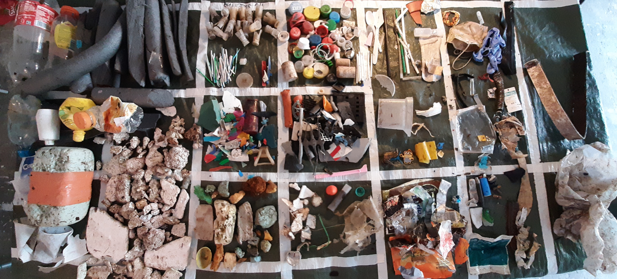
Below: Different sampling environments

The length and width of the survey area is measured at each survey. Thus, the number of items can be reported in a standard unit indifferent of the survey locations. In this report the standard reporting unit recommended by the EU is used: pieces of litter per 100 meters.

14.1.2.2. Counting objects¶

All visible objects within a survey area are collected, classified and counted. Total material and plastic weights are also recorded. Items are classified by code definitions based on a master list of codes in The Guide. Specific objects that are of local interest have been added under G9xx and G7xx.

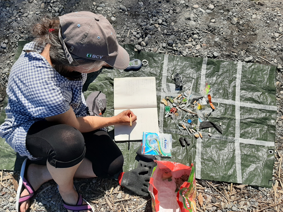
Below: Counting and classifying a sample. The objects are sorted and counted after collection. The original count is maintained in a notebook and the data is entered into the application, plages-propres at the convenience of the surveyor.

14.2. Calculating baselines¶

The methods described in sections 3 and 4 of A European Threshold Value and Assessment Method for Macro Litter on Coastlines and sections 6, 7 and 8 from Analysis of a pan-European 2012-2016 beach litter data set are applied to the beach litter survey results from April 2020 to May 2021.

The different options for calculating baselines, determining confidence intervals and identifying extreme values are explained and examples are given.

Assumptions:

The more litter on the ground, the more a person is likely to find
The survey results represent the minimum amount of litter at that site
For each survey: finding one item does not effect the chance of finding another

14.2.1. The data¶

Only surveys with a length greater than ten meters and are included in the baseline calculation. The following objects were excluded:

Objects less than 2.5cm
Paraffin, wax, oil and other pollutants

# define the final survey data set here:
a_data = survey_data.copy()

a_data = a_data[a_data.river_bassin != 'les-alpes']

# make a loc_date column from the survey data
# before converting to timestamp
a_data['loc_date']=tuple(zip(a_data.location, a_data.date))

# convert string dates from .csv to timestamp
a_data['date']=pd.to_datetime(a_data['date'], format='%Y-%m-%d')

# slice by start - end date
a_data = a_data[(a_data.date >= start_date)&(a_data.date <= end_date)]

# combine lugano and maggiore
# if the river bassin name does not equal tresa leave it, else change it to ticino
a_data['river_bassin'] = a_data.river_bassin.where(a_data.river_bassin != 'tresa', 'ticino' )

# assign the reporting value
a_data[unit_label] = (a_data.pcs_m * reporting_unit).round(2)

# save the data before aggregating to test
before_agg = a_data.copy()

# !! Remove the objects less than 2.5cm and chemicals !!
codes_todrop = ['G81', 'G78', 'G212', 'G213', 'G214']
a_data = a_data[~a_data.code.isin(codes_todrop)]

# use the code groups to get rid of all objects less than 5mm
a_data = a_data[a_data.groupname !=  'micro plastics (< 5mm)']

# match records to survey data
fd_dims= dfDims[(dfDims.location.isin(a_data.location.unique()))&(dfDims.date >= start_date)&(dfDims.date <= end_date)].copy()

# make a loc_date column and get the unique values
fd_dims['loc_date'] = list(zip(fd_dims.location, fd_dims.date))

# map the survey area name to the dims data record
a_map = fd_dims[['loc_date', 'area']].set_index('loc_date')
l_map = fd_dims[['loc_date', 'length']].set_index('loc_date')

# map length and area from dims to survey data
for a_survey in fd_dims.loc_date.unique():
    a_data.loc[a_data.loc_date == a_survey, 'length'] = l_map.loc[[a_survey], 'length'][0]
    a_data.loc[a_data.loc_date == a_survey, 'area'] = a_map.loc[[a_survey], 'area'][0]

# exclude surveys 10 meters or less
fd = a_data.loc[(a_data.length > 10)].copy()

# this is a common aggregation
agg_pcs_quantity = {unit_label:'sum', 'quantity':'sum'}

# survey totals by location
dt_all = fd.groupby(['loc_date','location','river_bassin', 'water_name_slug','date'], as_index=False).agg(agg_pcs_quantity)

Below: Survey results and summary statistics: samples greater than 10m and excluding objects less than 2.5cm and chemicals, n=372

# palettes and labels
bassin_pallette = {'rhone':'dimgray', 'aare':'salmon', 'linth':'tan', 'ticino':'steelblue', 'reuss':'purple'}
comp_labels = {"linth":"Linth/Limmat", "rhone":"Rhône", 'aare':"Aare", "ticino":"Ticino/Cerisio", "reuss":"Reuss"}
comp_palette = {"Linth/Limmat":"dimgray", "Rhône":"tan", "Aare":"salmon", "Ticino/Cerisio":"steelblue", "Reuss":"purple"}

# months locator, can be confusing
# https://matplotlib.org/stable/api/dates_api.html
months = mdates.MonthLocator(interval=1)
months_fmt = mdates.DateFormatter('%b')
days = mdates.DayLocator(interval=7)

# sns.set_style('whitegrid')

fig = plt.figure(figsize=(8,5))

gs = GridSpec(1,5)

ax = fig.add_subplot(gs[:,0:3])
axtwo = fig.add_subplot(gs[:, 3:])

# scale the chart as needed to accomodate for extreme values
scale_back = 98

# the results gets applied to the y_limit function in the chart
the_90th = np.percentile(dt_all[unit_label], scale_back)

# the survey totals
sns.scatterplot(data=dt_all, x='date', y=unit_label, hue='river_bassin', palette=bassin_pallette, alpha=1, ax=ax)

# set params on ax:
ax.set_ylim(0,the_90th )
ax.set_ylabel(unit_label, **ck.xlab_k14)

ax.set_xlabel("")
ax.xaxis.set_minor_locator(days)
ax.xaxis.set_major_formatter(months_fmt)

# axtwo
a_color = "dodgerblue"

# summarize the survey totals and format for printing
table_data = dt_all[unit_label].describe()
table_data.drop('count', inplace=True)
table_data = table_data.astype('int')
table_data = table_data.map(lambda x: "{:,}".format(x))

# make a 2d array
t_data = list(zip(table_data.index, table_data.values))

sut.hide_spines_ticks_grids(axtwo)

table_one = sut.make_a_table(axtwo, t_data,  colLabels=["Stat", unit_label], colWidths=[.5,.5], bbox=[0, 0, 1, 1])
# table_three = sut.make_a_table(axtwo, fd_mat_t,  colLabels=list(cols_to_use.values()), colWidths=[.4, .3,.3],  bbox=[0,0,1,1], **{"loc":"lower center"})
# a_summary_table_one = sut.make_a_summary_table(the_first_table_data,t_data,["Stat", unit_label], a_color, s_et_bottom_row=True)
table_one.get_celld()[(0,0)].get_text().set_text(" ")
# a_summary_table_one.set_fontsize(14)

axtwo.tick_params(which='both', axis='both', labelsize=14)
ax.tick_params(which='both', axis='both', labelsize=14)
ax.grid(visible=True, which='major', axis='y', linestyle='-', linewidth=1, c='black', alpha=.1, zorder=0)

plt.tight_layout()
plt.show()
plt.close()

Below: Distribution of surveys and percentile ranking values: all surveys. Note the mean (341p/100m) is greater than the median (180p/100m).

# percentile rankings  1, 5, 10, 15, 20
these_vals = []
for element in [.01,.05,.10,.15,.20, .5, .9 ]:
    a_val = np.quantile(dt_all[unit_label].to_numpy(), element)
    these_vals.append((F"{element*100}%",F"{int(a_val)}"))
    


fig = plt.figure(figsize=(10,5))

gs = GridSpec(1,5)

ax = fig.add_subplot(gs[:,0:3])
axtwo = fig.add_subplot(gs[:, 3:])
ax.grid(visible=True, which='major', axis='y', linestyle='-', linewidth=1, c='black', alpha=.1, zorder=0)

sns.histplot(data=dt_all, x=unit_label, stat='count', ax=ax, alpha=0.6)
ax.axvline(x=dt_all[unit_label].median(), c='magenta', label='median')
ax.axvline(x=dt_all[unit_label].mean(), c='red', label='mean')
ax.legend()

sut.hide_spines_ticks_grids(axtwo)

# the_first_table_data = axtwo.table(these_vals,  colLabels=('ranking', unit_label), colWidths=[.5,.5], bbox=[0, 0, 1, 1])

table_two = sut.make_a_table(axtwo, these_vals, colLabels=('ranking', unit_label), colWidths=[.5,.5], bbox=[0, 0, 1, 1])
table_two.get_celld()[(0,0)].get_text().set_text("ranking")
table_two.set_fontsize(14)

axtwo.tick_params(which='both', axis='both', labelsize=14)
ax.tick_params(which='both', axis='both', labelsize=14)
plt.show()

14.2.2. The assessment metric¶

Calculating baseline values requires the aggregation of survey results at different temporal and geographic scales. The best method is:

Robust with respect to outliers
Simple to calculate
Widely understood

The two most common test statistics used to compare data are the mean and the median. The mean is the best predictor of central tendency if the data are \(\approxeq\) normally distributed. However, beach litter survey results have a high variance relative to the mean. Methods can be applied to the data to reduce the effects of high variance when calculating the mean:

trimmed mean: removes a small, designated percentage of the largest and smallest values before calculating the mean
tri mean: the weighted average of the median and upper and lower quartiles, \((Q1 + 2Q2 + Q3)/4\)
mid hinge: \((Q1 + Q3)/2\)

While effective at reducing the effects of the outliers, the previous methods are not as simple to calculate as the mean or the median and therefore the significance of the results may not be well understood.

The median (50th percentile) is an equally good predictor of the central tendency but is much less effected by extreme values compared to the mean. The more a set of data approaches a normal distribution the closer the median and mean approach. The median and the accompanying percentile functions are available on most spreadsheet applications.

For the reasons cited previously, the median value of a minimum number of samples collected from a survey area during one sampling period is considered statistically suitable for beach litter assessments. For the marine environment the *minimum number of samples is 40 per subregion and the sampling period is 6 years. [HG19]

14.2.3. Confidence intervals (CIs)¶

Confidence intervals (CIs) help communicate the uncertainty of beach-litter survey results with regards to any general conclusions that may be drawn about the abundance of beach litter within a region. The CI gives the lower and higher range of the estimate of the test statistic given the sample data.

The best way to mitigate uncertainty is to have the appropriate number of samples for the region or area of interest. However, beach litter surveys have a high variance and any estimate of an aggregate value should reflect that variance or uncertainty. CIs provide a probable range of values given the uncertainty/variance of the data.[HG19]

In this method data is NOT excluded from the baseline calculations and confidence intervals:

It was agreed to leave the extreme results in the dataset, while highlighting the need to check to verify extreme data case by case and to apply the median for calculating of averages. This allows the use of all data while not skewing results through single extraordinary high litter count surveys. [VLW20]

14.2.3.1. Bootstrap methods:¶

Bootstrapping is a resampling method that uses random sampling with replacement to repeat or simulate the sampling process. Bootstrapping permits the estimation of the sampling distribution of sample statistics using random sampling methods. [Wika] [JLGC19] [Sta21b]

Bootstrap methods are used to calculate the CIs of the test statistics, by repeating the sampling process and evaluating the median at each repetition. The range of values described by the middle 95% of the bootstrap results is the CI for the observed test statistic.

There are several computational methods to choose from such as percentile, BCa, and Student’s t. For this example, two methods were tested:

Percentile bootstrap
Bias-corrected accelerated bootstrap confidence interval (BCa)

The percentile method does not account for the shape of the underlying distribution, and this can lead to confidence intervals that do not match the data. The BCa corrects that. The implementation of these methods is straight forward using the previously cited packages. [Efr87] [dry20] [Boi19]

14.2.4. Comparing bootstrap CIs¶

# this code was modified from this source:
# http://bebi103.caltech.edu.s3-website-us-east-1.amazonaws.com/2019a/content/recitations/bootstrapping.html
# if you want to get the confidence interval around another point estimate use np.percentile
# and add the percentile value as a parameter

def draw_bs_sample(data):
    """Draw a bootstrap sample from a 1D data set."""
    return np.random.choice(data, size=len(data))

def compute_jackknife_reps(data, statfunction=None, stat_param=False):
    '''Returns jackknife resampled replicates for the given data and statistical function'''
    # Set up empty array to store jackknife replicates
    jack_reps = np.empty(len(data))

    # For each observation in the dataset, compute the statistical function on the sample
    # with that observation removed
    for i in range(len(data)):
        jack_sample = np.delete(data, i)
        if not stat_param:
            jack_reps[i] = statfunction(jack_sample)
        else:
            jack_reps[i] = statfunction(jack_sample, stat_param)          
        
    return jack_reps


def compute_a(jack_reps):
    '''Returns the acceleration constant a'''

    mean = np.mean(jack_reps)
    try:
        a = sum([(x**-(i+1)- (mean**-(i+1)))**3 for i,x in enumerate(jack_reps)])
        b = sum([(x**-(i+1)-mean-(i+1))**2 for i,x in enumerate(jack_reps)])
        c = 6*(b**(3/2))
        data = a/c
    except:
        print(mean)
    return data


def bootstrap_replicates(data, n_reps=1000, statfunction=None, stat_param=False):
    '''Computes n_reps number of bootstrap replicates for given data and statistical function'''
    boot_reps = np.empty(n_reps)
    for i in range(n_reps):
        if not stat_param:
            boot_reps[i] = statfunction(draw_bs_sample(data))
        else:
            boot_reps[i] = statfunction(draw_bs_sample(data), stat_param)     
        
    return boot_reps


def compute_z0(data, boot_reps, statfunction=None, stat_param=False):
    '''Computes z0 for given data and statistical function'''
    if not stat_param:
        s = statfunction(data)
    else:
        s = statfunction(data, stat_param)
    return stats.norm.ppf(np.sum(boot_reps < s) / len(boot_reps))


def compute_bca_ci(data, alpha_level, n_reps=1000, statfunction=None, stat_param=False):
    '''Returns BCa confidence interval for given data at given alpha level'''
    # Compute bootstrap and jackknife replicates
    boot_reps = bootstrap_replicates(data, n_reps, statfunction=statfunction, stat_param=stat_param)
    jack_reps = compute_jackknife_reps(data, statfunction=statfunction, stat_param=stat_param)

    # Compute a and z0
    a = compute_a(jack_reps)
    z0 = compute_z0(data, boot_reps, statfunction=statfunction, stat_param=stat_param)

    # Compute confidence interval indices
    alphas = np.array([alpha_level/2., 1-alpha_level/2.])
    zs = z0 + stats.norm.ppf(alphas).reshape(alphas.shape+(1,)*z0.ndim)
    avals = stats.norm.cdf(z0 + zs/(1-a*zs))
    ints = np.round((len(boot_reps)-1)*avals)
    ints = np.nan_to_num(ints).astype('int')

    # Compute confidence interval
    boot_reps = np.sort(boot_reps)
    ci_low = boot_reps[ints[0]]
    ci_high = boot_reps[ints[1]]
    return (ci_low, ci_high)

quantiles = [.1, .2, .5, .9]
q_vals = {x:dt_all[unit_label].quantile(x) for x in quantiles}

the_bcas = {}
for a_rank in quantiles:
    an_int = int(a_rank*100)
    a_result = compute_bca_ci(dt_all[unit_label].to_numpy(), .05, n_reps=5000, statfunction=np.percentile, stat_param=an_int)
    observed = np.percentile(dt_all[unit_label].to_numpy(), an_int)
    the_bcas.update({F"{int(a_rank*100)}":{'2.5% ci':a_result[0], 'observed': observed, '97.5% ci': a_result[1]}})


bca_cis = pd.DataFrame(the_bcas)
bcas = bca_cis.reset_index()
bcas[['10', '20', '50', '90']] = bcas[['10', '20', '50', '90']].astype('int')
bcas['b-method'] = 'BCa'

# bootstrap percentile confidence intervals
# resample the survey totals for n times to help
# define the range of the sampling statistic
# the number of reps
n=5000

# keep the observed values
observed_median = dt_all[unit_label].median()
observed_tenth = dt_all[unit_label].quantile(.15)

the_cis = {}

for a_rank in quantiles:
    # for the median
    sim_ptile = []

    # for the tenth percentile
    sim_ten = []
    for element in np.arange(n):
        less = dt_all[unit_label].sample(n=len(dt_all), replace=True)    
        a_ptile = less.quantile(a_rank)
        sim_ptile.append(a_ptile)
    # get the upper and lower range of the test statistic disrtribution:
    a_min = np.percentile(sim_ptile, 2.5)
    a_max = np.percentile(sim_ptile, 97.5)
    
    # add the observed value and update the dict
    the_cis.update({F"{int(a_rank*100)}":{'2.5% ci':a_min, 'observed': q_vals[a_rank], '97.5% ci': a_max}})

# make df
p_cis = pd.DataFrame(the_cis)
p_cis = p_cis.astype("int")
p_cis['b-method'] = '%'
p_cis.reset_index(inplace=True)

Below top: Confidence intervals calculated by resampling the survey results 5,000 times for each condition. Below bottom: The same intervals using the bias corrected method.

fig, axs = plt.subplots(2,1, figsize=(8,8))
axone = axs[0]
axtwo = axs[1]

data = p_cis.values
sut.hide_spines_ticks_grids(axone)
sut.hide_spines_ticks_grids(axtwo)
colLabels = ["$" + F"{x}" +"^{th}$" for x in p_cis.columns[:-1]]
colLabels.append('method')

table_one = sut.make_a_table(axone, data, colLabels=colLabels, colWidths=[.25,*[.15]*5], bbox=[0, 0, 1, 1])
table_two = sut.make_a_table(axtwo, bcas.values, colLabels=colLabels, colWidths=[.25,*[.15]*5], bbox=[0, 0, 1, 1])

table_one.set_fontsize(14)
table_two.set_fontsize(14)    
                        
table_one.get_celld()[(0,0)].get_text().set_text("Percentile")
table_two.get_celld()[(0,0)].get_text().set_text("BCa")

plt.tight_layout()
plt.subplots_adjust(hspace=.2)
plt.show()
plt.close()

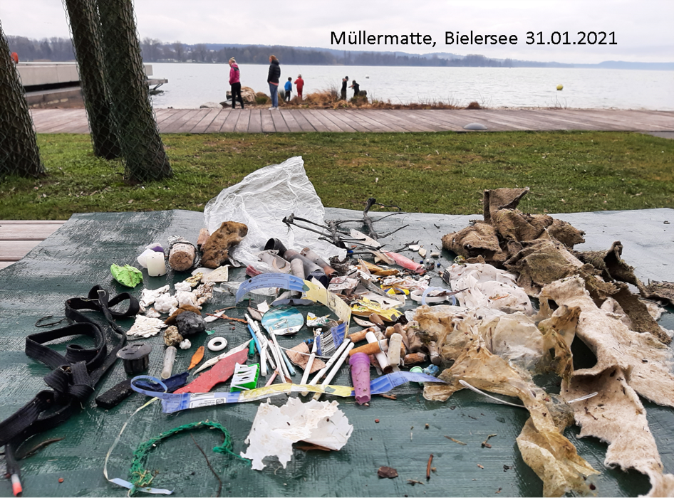
Below: Confidence interval example value: the survey result at Biel on 31-01-2021 was greater than the median value for all the surveys, it exceeded the the confidence interval of the the 50^th percentile. There were 123 objects (pcs) collected over 40 meters (m) of shoreline. First the survey value is converted to pieces of litter per meter (pcs/m) and then multiplied by the required number of meters (100).

\((pcs/m)*100 = (123_{pcs} / 40_m)*100m \approxeq 313p/100m\)

14.2.5. Baseline values¶

For this set of data, the differences between the CIs calculated the BCa method or the percentile method is minimum. The BCa method will be used to report the baseline values and CIs.

14.2.5.1. Baseline median value of all survey results¶

Considering only surveys with a length greater than 10 meters and excluding objects less than 2.5cm, the median survey result of all data was 180p/100m with a CI of 147p/100m - 212p/100m. The reported baseline median value for the EU was 133p/100m, within the range of the CI of the IQAASL survey results. While the median value may be greater in Switzerland the mean value from the EU study is 504p/100m versus 341p/100m in Switzerland.[HG19]

Suggesting that the higher extreme values were more likely in marine environment, but the expected median value from both data sets is similar.

14.2.5.2. Baseline median and CI per survey area¶

There were four survey areas in the IQAASL, 3 of which had more than 40 samples during the survey period.

Below: The median and the 95% confidence interval of the Linth, Aare and Rhône survey areas. The Ticino survey area is not included for lack of a sufficient quantity of surveys.

bassins = ["linth", "aare", "rhone"]
the_sas = {}
for a_bassin in bassins:
    an_int = int(a_rank*100)
    a_result = compute_bca_ci(dt_all[dt_all.river_bassin == a_bassin][unit_label].to_numpy(), .05, n_reps=5000, statfunction=np.percentile, stat_param=50)
    observed = np.percentile(dt_all[dt_all.river_bassin == a_bassin][unit_label].to_numpy(), 50)
    the_sas.update({a_bassin:{'2.5% ci':a_result[0], 'observed': observed, '97.5% ci': a_result[1]}})

sas = pd.DataFrame(the_sas)
sas['b-method'] = 'bca'
sas = sas.reset_index()

fig, axs = plt.subplots(figsize=(7,4))

data = sas.values
sut.hide_spines_ticks_grids(axs)

# the_first_table_data = axs.table(data, colLabels=sas.columns, colWidths=[.25,*[.15]*5], bbox=[0, 0, 1, 1])

table_one = sut.make_a_table(axs, data, colLabels=sas.columns, colWidths=[.25,*[.15]*5], bbox=[0, 0, 1, 1])

table_one.get_celld()[(0,0)].get_text().set_text(" ")

table_one.set_fontsize(14)

plt.show()
plt.close()

14.3. Extreme values¶

As was noted earlier, extreme values (EVs) or outliers are not excluded from the data when calculating baselines or CIs. However, identifying EVs and where and when they occur is an essential part of the monitoring process.

The occurrence of extreme values can influence the average of the data and the interpretation of survey results. According to the JRC report:

The methodology for the identification of extreme values can be either expert judgement, or be based on statistical and modelling approaches, such as the application of Tukey’s box plots to detect potential outliers. For skewed distributions, the adjusted box plot is more appropriate. [HG19]

14.3.1. Defining extreme values¶

The references give no guidance as to the numerical value of an EV. Contrary to the target value of 20p/100m or the \(15^{th}\) percentile, the definition of an EV is left to the person interpreting the data. The upper limit of Tukeys boxplots (un adjusted) is \(\approx 90^{th}\) percentile of the data. This method is compatible with the assessment metric and boxplots are fairly easy to resolve visually.

14.3.1.1. Adjusted boxplots¶

Tukey’s boxplot is used to visualize the distribution of a univariate data set. The samples that fall within the first quartile (25%) and the third quartile (75%) are considered to be within the inner quartile range (IQR). Points out side of the inner quartile range are considered outliers if their value is greater or less than one of two limits:

lower limit = \(Q_1 - (1.5*IQR)\)
upper limit = \(Q_3 + (1.5*IQR)\)

Adjusting the boxplot involves replacing the constant 1.5 with another parameter. This parameter is calculated using a method called the medcouple (MC) and applying the result of that method to the constant 1.5. [HV08] [SP] The new calculation looks like this:

lower limit = \(Q_1 - (1.5e^{-4MC}*IQR)\)
upper limit = \(Q_3 + (1.5e^{3MC}*IQR)\)

The limits are extended or reduced to better match the shape of the data. As a result, the upper and lower limits represent a wider range of values, with respect to the percentile ranking, as opposed to the unadjusted version.

Below: The limit at which a survey is considered extreme extends to the 98th percentile when the boxplots are adjusted as opposed to the 90th percentile if the constant is left at 1.5.

# implementation of medcouple
a_whis = medcouple(dt_all[unit_label].to_numpy())

# get the ecdf 
ecdf = ECDF(dt_all[unit_label].to_numpy())

# quantiles and IQR of the data
q1 = dt_all[unit_label].quantile(0.25)
q3 =dt_all[unit_label].quantile(0.75)
iqr = q3 - q1

# the upper and lower limit of extreme values unadjusted:
limit_lower = q1 - 1.5*iqr
limit_upper = q3 + 1.5*iqr

# the upper and lower limit of extreme values adjusted:
a_fence = q1 - (1.5*(math.exp((-4*a_whis))))*iqr
a_2fence = q3 + (1.5*(math.exp((3*a_whis))))*iqr

fig, ax = plt.subplots(figsize=(4,6))
box_props = {
    'boxprops':{'facecolor':'none', 'edgecolor':'magenta'},
    'medianprops':{'color':'magenta'},
    'whiskerprops':{'color':'magenta'},
    'capprops':{'color':'magenta'}
}

sns.stripplot(data=dt_all, y=unit_label, ax=ax, zorder=1, color='black', jitter=.35, alpha=0.3, s=8)
sns.boxplot(data=dt_all, y=unit_label, ax=ax, zorder=3, orient='v', showfliers=False, **box_props)
ax.axhline(y=a_2fence, xmin=.25, xmax=.75, c='magenta', zorder=3,)
ax.set_ylabel(unit_label, **ck.xlab_k14)

ax.tick_params(which='both', axis='both', labelsize=14)
ax.tick_params(which='both', axis='x', bottom=False)

ax.set_ylim(0, a_2fence+200)

ax.annotate("Adjusted",
                  xy=(0, a_2fence), xycoords='data',
                  xytext=(.2,a_2fence-400), textcoords='data',
                  size=14, va="center", ha="center",
                  bbox=dict(boxstyle="round4", fc="w", alpha=0.1),
                  arrowprops=dict(arrowstyle="-|>",
                                  connectionstyle="arc3,rad=-0.2",
                                  fc="black"),)

ax.annotate("Not Adjusted",
                  xy=(0, limit_upper), xycoords='data',
                  xytext=(-.2,limit_upper+400), textcoords='data',
                  size=14, va="center", ha="center",
                  bbox=dict(boxstyle="round4", fc="w",alpha=0.5),
                  arrowprops=dict(arrowstyle="-|>",
                                  connectionstyle="arc3,rad=-0.2",
                                  fc="black"),)
ax.grid(visible=True, which='major', axis='y', linestyle='-', linewidth=1, c='black', alpha=.1, zorder=0)

plt.show()

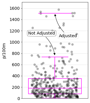
The difference between adjusted and normal boxplots. Adjusted = 1507 p/100m, unadjusted = 755 p/100m.

Using the adjusted boxplots pushes the extreme value threshold (EVT) to over 1600p/100m. However, the unadjusted boxplots fall within the CI of the expected value of the 90^th percentile of the survey data.

Below: adjusted extreme values example St. Gingolph, 08-12-2020. There were 514 objects (pcs) collected over 31 meteres (m) of shoreline. First the survey value is converted to pieces of trash per meter (pcs/m) and then multiplied by the required number of meters (100):

\((pcs/m)*100 = (514_{pcs} / 31_m)*100m \approxeq 1652p/100m\)

14.3.1.2. Modeling¶

Extreme values can be identified by assuming the data belong to some underlying known statistical distribution. In general count data are assumed to be Poisson distributed or a form very similar. The Poisson distribution assumes that the mean = the variance. The data from IQAASL and beach-litter data in general have a high variance usually greater than the mean.

The negative binomial (NB) distribution does not have such a requirement. The NB is a Poisson distribution with parameter λ, where λ itself is not fixed but a random variable which follows a Gamma distribution. [CT99] [Wei20] [nbi]

The modelling approach for the identification of extreme values is then performed by fitting the NB-distribution to the data by means of maximum likelihood (MLE) and tagging all values in the right tail as potentially extreme values if the probability that they belong to the fitted NB-distribution is less than, e.g. 0.001. [VLW20]

The MLE is one of two recommended methods of modeling or fitting data values to an assumed distribution:

Method of moments (MOM)
MLE: maximum likelihood estimation

14.3.1.2.1. Method of moments¶

The method of moments assumes that the parameters derived from the sample are close or similar to the population parameters. In the case of beach-litter surveys that means the sample median, mean and variance could be considered close approximations of the actual values if all the beaches on all the lakes and streams were surveyed.

Concretely, the parameters of a probable distribution model are estimated by calculating them from the sample data. This method is easy to apply because most of the parameter calculations for the most common distributions are well known. [MDG18] [VGO+20] [SO]

14.3.1.2.2. Maximum likelihood estimation¶

MLE is a method of estimating the parameters of a statistical model given some data, in that way it is not different than the MOM. The difference is that in the MOM the model parameters are calculated from the data, in MLE the parameters are chosen by finding the parameters that make the data most likely given the statistical model.

This method is more computationally involved than the MOM but has some advantages:

If the model is correctly assumed, the MLE is the most efficient estimator.
It results in unbiased estimates in larger samples.

Fitting the data to the underlying NB distribution. The observed survey results are compared to the estimated survey results using the method of moments and maximum likelihood estimation. Left: histogram of simulated results compared to observed data. Right: distribution of results compared to observed data with the 90^th percentile.

# implementaion of MLE
# https://github.com/pnxenopoulos/negative_binomial/blob/master/negative_binomial/core.py

def r_derv(r_var, vec):
    ''' Function that represents the derivative of the negbinomial likelihood
    '''

    total_sum = 0
    obs_mean = np.mean(vec)  # Save the mean of the data
    n_pop = float(len(vec))  # Save the length of the vector, n_pop

    for obs in vec:
        total_sum += digamma(obs + r_var)

    total_sum -= n_pop*digamma(r_var)
    total_sum += n_pop*math.log(r_var / (r_var + obs_mean))

    return total_sum

def p_equa(r_var, vec):
    ''' Function that represents the equation for p in the negbin likelihood
     '''
    data_sum = sum(vec)
    n_pop = float(len(vec))
    p_var = 1 - (data_sum / (n_pop * r_var + data_sum))
    return p_var

def neg_bin_fit(vec, init=0.0001):
    ''' Function to fit negative binomial to data
    vec: the data vector used to fit the negative binomial distribution
   
    '''
    est_r = newton(r_derv, init, args=(vec,))
    est_p = p_equa(est_r, vec)
    return est_r, est_p

# the data to model
vals = dt_all[unit_label].to_numpy()

# the variance
var = np.var(vals)

# the average
mean = np.mean(vals)

# dispersion
p = (mean/var)
n = (mean**2/(var-mean))

# implementation of method of moments
r = stats.nbinom.rvs(n,p, size=len(vals))

# format data for charting
df = pd.DataFrame({unit_label:vals, 'group':'observed'})
df = pd.concat([df,pd.DataFrame({unit_label:r, 'group':'MOM'})])

scp = df[df.group == 'MOM'][unit_label].to_numpy()
obs = df[df.group == 'observed'][unit_label].to_numpy()

scpsx = [{unit_label:x, 'model':'MOM'} for x in scp]
obsx = [{unit_label:x, 'model':'observed'} for x in obs]

# ! implementation of MLE
estimated_r, estimated_p = neg_bin_fit(obs, init = 0.0001)

# ! use the MLE estimators to generate data
som_data = stats.nbinom.rvs(estimated_r, estimated_p, size=len(dt_all))
som_datax = pd.DataFrame([{unit_label:x, 'model':'MLE'}  for x in som_data])

# combined the different results in to one df
data = pd.concat([pd.DataFrame(scpsx), pd.DataFrame(obsx), pd.DataFrame(som_datax)])
data.reset_index(inplace=True)

# the 90th
ev = data.groupby('model', as_index=False)[unit_label].quantile(.9)
xval={'MOM':0, 'observed':1, 'MLE':2}
ev['x'] = ev.model.map(lambda x: xval[x])
box_palette = {'MOM':'salmon', 'MLE':'magenta', 'observed':'dodgerblue'}

fig, axs = plt.subplots(1,2, figsize=(10,6))

ax=axs[0]
axone=axs[1]

bw=80

sns.histplot(data=data, x=unit_label, ax=ax, hue='model', zorder=2, palette=box_palette, binwidth=bw, element='bars', multiple='stack', alpha=0.4)

box_props = {
    'boxprops':{'facecolor':'none', 'edgecolor':'black'},
    'medianprops':{'color':'black'},
    'whiskerprops':{'color':'black'},
    'capprops':{'color':'black'}
}


sns.boxplot(data=data, x='model', y=unit_label, ax=axone, zorder=5, palette=box_palette, showfliers=False, dodge=False, **box_props)
sns.stripplot(data=data, x='model', y=unit_label, hue='model', zorder=0,palette=box_palette, ax=axone, s=8, alpha=0.2, dodge=False, jitter=0.4)
axone.scatter(x=ev.x.values, y=ev[unit_label].values, label="90%", color='black', s=60)
axone.set_ylim(0,np.percentile(r, 95))
ax.get_legend().remove()
ax.set_ylabel("Number of samples", **ck.xlab_k14)
axone.set_ylabel(unit_label, **ck.xlab_k14)

handles, labels = axone.get_legend_handles_labels()
axone.get_legend().remove()
h3=handles[:3]
hlast= handles[-1:]
axone.set_xlabel("")
axone.tick_params(which='both', axis='both', labelsize=14)
ax.tick_params(which='both', axis='both', labelsize=14)
l3 = labels[:3]
llast = labels[-1:]

ax.grid(visible=True, which='major', axis='y', linestyle='-', linewidth=1, c='black', alpha=.2, zorder=0)
axone.grid(visible=True, which='major', axis='y', linestyle='-', linewidth=1, c='black', alpha=.2, zorder=0)


fig.legend([*h3, *hlast], [*l3, *llast], bbox_to_anchor=(.48, .96), loc='upper right', fontsize=14)
plt.tight_layout()
plt.show()

evx = ev.set_index('model')

pnt =  F"""*90% p/100m: &nbsp;MLE={evx.loc['MLE'][unit_label].astype('int')},  &nbsp;Observed={evx.loc['observed'][unit_label].astype('int')},  &nbsp;MOM={evx.loc['MOM'][unit_label].astype('int')}*"""
md(pnt)

90% p/100m: MLE=826, Observed=727, MOM=951

14.4. Implementation¶

The proposed, assessment metrics and evaluation methods for beach litter survey results are similar and compatible with the methods previously implemented in Switzerland. This first analysis has shown that:

Methods proposed by the EU to monitor litter are applicable in Switzerland
Confidence intervals and baselines can be calculated for different survey areas
Aggregated results can be compared between regions

Once the BV for a survey area is calculated all samples that are conducted within that survey area can be compared directly to it. It is the case in 2020 - 2021 that the survey areas in Switzerland have different median baselines. This situation is analogous to the EU with respect to the differences between different regions and administrative areas of the continent.

By applying the proposed methods to the current results from IQAASL the objects of concern can be identified for each survey area.

Below: Comparing the baseline values of the most common objects. All survey areas 2020 - 2021. The Ticino/Cerisio survey area has less than 100 surveys. units= p/100m

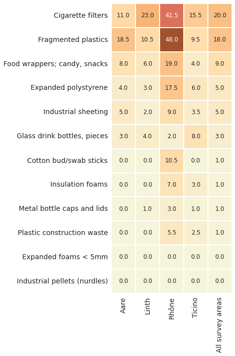
The expected median value per survey and the median value of the most common objects per survey is higher in the Rhône survey area. When the median value is used the BV also reveals that 2/12 most common objects were found in less than 50% of the surveys nationally, those with a median value of zero.

The method can be scaled vertically giving a more detailed view of a survey area. The method of calculation remains the same therefore comparisons are valid from the lake to the national level.

Below: Comparing the baseline values of the most common objects. Aare survey area lakes and rivers 2020 - 2021. Locations with more than 30 surveys: Bielersee, Neuenburgersee and Thunersee.

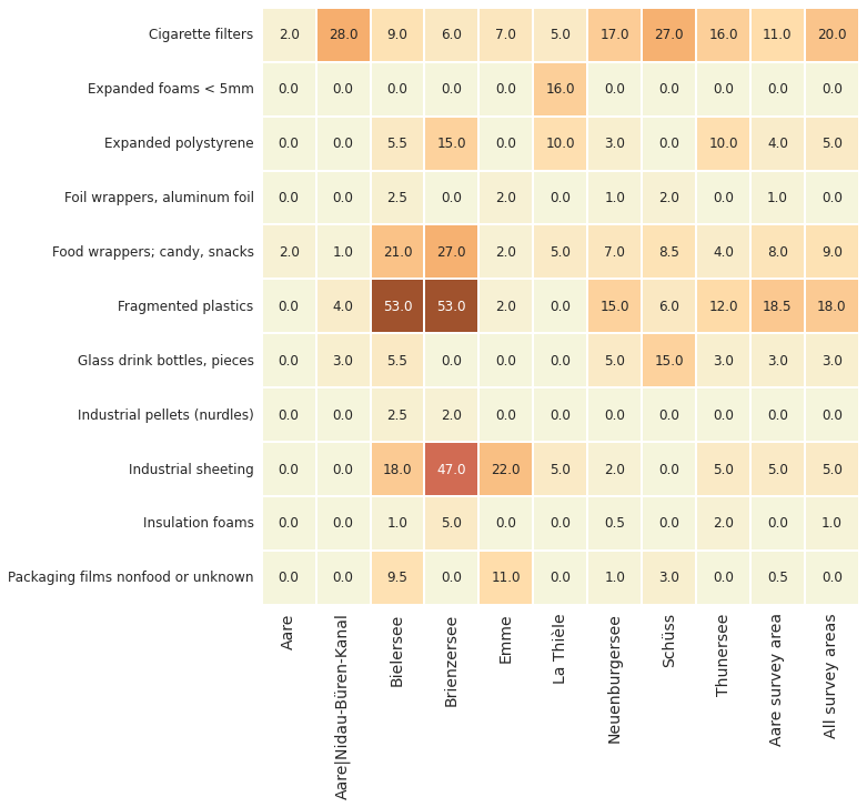
The recommended minimum number of surveys (40) per sampling period is to ensure that BV calculations are based on enough samples, this is important because of the high variability of beach litter surveys.

The sampling period for IQAASL was March through May 2020 - 2021. With respect to the minimum number of samples there are three baseline values for the Aare survey area:

Bielersee
Neuenburgersee
The Aare survey area

For assessment purposes this means that one sample can serve as a spot assessment and the results can be compared to any of the regional baselines directly, providing instant feedback. This type of assessment simplifies the process and empowers local stakeholders to carry out independent assessments, draw conclusions and define mitigation strategies based on the results of the established BV for the survey area.

In the previous examples no threshold values or extreme values are indicated. Values greater than zero are the expected median amount of that object for every measured unit. A zero value indicates that the object was found in less than 50% of the surveys. The percentile ranking for a particular object can be inferred by reading the table of values in the horizontal direction.

How meaningful these results are to the assessment of mitigation strategies depends on the number and quality of samples. Stakeholders at the municipal or local level need detailed data about specific objects. While national and international stakeholders tend to use broader aggregated groups.

The quality of the data is directly related to the training and support of the surveyors. The identification process requires some expertise as many objects and materials are not familiar to the average person. A core team of experienced surveyors to assist in the development and training ensures surveys are conducted consistently over time.

The monitoring program in Switzerland has managed to keep pace with developments on the continent, there are however many areas of improvement:

Defining a standardized reporting method for municipal, cantonal and federal stakeholders
Define monitoring or assessment goals
Formalize the data repository and the method for implementation at different administrative levels
Develop a network of associations that share the responsibility and resources for surveying the territory
Develop and implement a formal training program for surveyors
Determine, in collaboration with academic partners, ideal sampling scenarios and research needs
Develop a financing method to conduct the recommended minimum number of surveys (40), per sampling period, per survey area to ensure accurate assessments can be made and research requirements are met.

Changes in beach-litter survey results are signals and using baseline values helps identify the magnitude of those signals. However, without any context or additional information these signals may appear random.

Expert judgment includes the ability to place survey results in the context of local events and topography. This capacity of discernment with regards to the data and the environment is essential to identifying potential sources and priorities.

Beach litter baselines

Contents