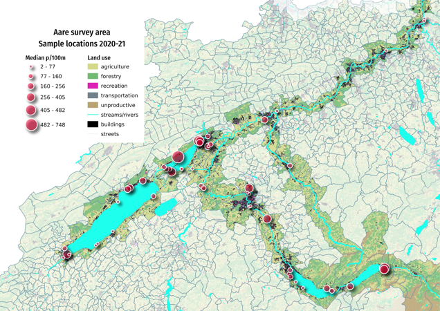
3. Aare¶

Below: Map of survey locations March 2020 - May 2021. Marker diameter = the mean survey result in pieces of litter per 100 meters (p/100m).

sut.display_image_ipython(bassin_map, thumb=(800,450))

3.1. Sample locations and land use characteristics¶

# this is the data before the expanded foams and fragmented plastics are aggregated to Gfrags and Gfoams
before_agg = pd.read_csv("resources/checked_before_agg_sdata_eos_2020_21.csv")

# this is the aggregated survey data that is being used
# a_data is all the data in the survey period
a_data = pd.read_csv(F"resources/checked_sdata_eos_2020_21.csv")
a_data["date"] = pd.to_datetime(a_data.date)

a_data.rename(columns={"% to agg":"% ag", "% to recreation": "% recreation", "% to woods":"% woods", "% to buildings":"% buildings"}, inplace=True)
luse_exp = ["% buildings", "% recreation", "% ag", "% woods", "streets km", "intersects"]

fd = sut.feature_data(a_data, this_feature["level"], these_features=[this_feature["slug"]])

# cumulative statistics for each code
code_totals = sut.the_aggregated_object_values(fd, agg=agg_pcs_median, description_map=code_description_map, material_map=code_material_map)    

# daily survey totals
dt_all = fd.groupby(["loc_date","location",this_level, "city","date"], as_index=False).agg(agg_pcs_quantity )

# the materials table
fd_mat_totals = sut.the_ratio_object_to_total(code_totals)

# summary statistics, nsamples, nmunicipalities, names of citys, population
t = sut.make_table_values(fd, col_nunique=["location", "loc_date", "city"], col_sum=["quantity"], col_median=[])

# make a map to the population values for each survey location/city
fd_pop_map = dfBeaches.loc[fd.location.unique()][["city", "population"]].copy()
fd_pop_map.drop_duplicates(inplace=True)

# update t with the population data
t.update(sut.make_table_values(fd_pop_map, col_nunique=["city"], col_sum=["population"], col_median=[]))

# update t with the list of locations from fd
t.update({"locations":fd.location.unique()})

# the lake and river names in the survey area
lakes = dfBeaches.loc[(dfBeaches.index.isin(t["locations"]))&(dfBeaches.water == "l")]["water_name"].unique()
rivers = dfBeaches.loc[(dfBeaches.index.isin(t["locations"]))&(dfBeaches.water == "r")]["water_name"].unique()

# join the strings into comma separated list
obj_string = "{:,}".format(t["quantity"])
surv_string = "{:,}".format(t["loc_date"])
pop_string = "{:,}".format(int(t["population"]))

# make strings
date_quantity_context = F"For the period between {start_date[:-3]} and {end_date[:-3]}, a total of {obj_string } objects were removed and identified over the course of {surv_string} surveys."
geo_context = F"The {bassin_label} results include {t['location']} different locations, {t['city']} different municipalities with a combined population of approximately {pop_string}."
# admin_context = F"There are {t['city']} different municipalities represented in these results with a combined population of approximately {pop_string}."
munis_joined = ", ".join(sorted(fd_pop_map["city"]))
lakes_joined = ", ".join(sorted(lakes))
rivers_joined = ", ".join(sorted(rivers))

# put that all together:
lake_string = F"""
{date_quantity_context} {geo_context }

*{bassin_label} lakes:*\n\n>{lakes_joined}

*{bassin_label} rivers:*\n\n>{rivers_joined}

*{bassin_label} municipalities:*\n\n>{munis_joined}
"""
md(lake_string)

For the period between 2020-03 and 2021-05, a total of 13,847 objects were removed and identified over the course of 140 surveys. The Aare survey area results include 51 different locations, 35 different municipalities with a combined population of approximately 493,799.

Aare survey area lakes:

Bielersee, Brienzersee, Neuenburgersee, Thunersee

Aare survey area rivers:

Aare, Aare|Nidau-Büren-Kanal, Emme, La Thièle, Schüss

Aare survey area municipalities:

Aarau, Beatenberg, Bern, Biel/Bienne, Boudry, Brienz (BE), Brugg, Brügg, Burgdorf, Bönigen, Cheyres-Châbles, Cudrefin, Erlach, Estavayer, Gals, Gebenstorf, Grandson, Hauterive (NE), Kallnach, Köniz, Le Landeron, Ligerz, Luterbach, Lüscherz, Neuchâtel, Nidau, Port, Rubigen, Solothurn, Spiez, Thun, Unterseen, Vinelz, Walperswil, Yverdon-les-Bains

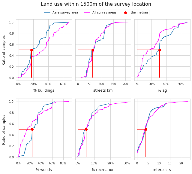
3.1.1. Land use profile of the surveys¶

The land use is reported as the percent of total area attributed to each land use category within a 1500m radius of the survey location.

Streets are reported as the total number of kilometers of streets within the 1500m radius. Intersects is also an ordinal ranking of the number of rivers/canals that intersect a lake within 1500m of the survey location.

The ratio of the number of samples under varying land use profiles gives an indication of the environmental and economic conditions of the survey sites.

For more information Land use profile

Below: Distribution of land use characteristics.

sns.set_style("whitegrid")
# the ratio of samples with respect to the different land use characteristics for each survey area
# the data to use is the unique combinations of loc_date and the land_use charcteristics of each location
project_profile = a_data[["loc_date", this_feature["level"], *luse_exp]].drop_duplicates()
dt_nw = fd[["loc_date", this_feature["level"], *luse_exp]].drop_duplicates()

# labels and levels
comps = [this_feature["slug"]]
comp_labels = {x:wname_wname.loc[x][0] for x in fd[this_level].unique()}

fig, axs = plt.subplots(2, 3, figsize=(9,8), sharey="row")

for i, n in enumerate(luse_exp):
    r = i%2
    c = i%3
    ax=axs[r,c]
    for element in[this_feature["slug"]]:
        data=dt_nw[dt_nw[this_feature["level"]] == element][n].values
        the_data = ECDF(data)
        
        # plot that
        sns.lineplot(x=the_data.x, y=the_data.y, ax=ax, label=bassin_label)
    
    # get the dist for all here
    a_all_surveys =  ECDF(project_profile[n].values)
    
    # plot that    
    sns.lineplot(x=a_all_surveys.x, y=a_all_surveys.y, ax=ax, label="All survey areas", color="magenta")
    
    # get the median from the data
    the_median = np.median(data)
    
    # plot the median and drop horzontal and vertical lines
    ax.scatter([the_median], 0.5, color="red",s=50, linewidth=2, zorder=100, label="the median")
    ax.vlines(x=the_median, ymin=0, ymax=0.5, color="red", linewidth=2)
    ax.hlines(xmax=the_median, xmin=0, y=0.5, color="red", linewidth=2)
    
    if i <= 3:
        if c == 0:            
            ax.set_ylabel("Ratio of samples", **ck.xlab_k)
        ax.xaxis.set_major_formatter(ticker.PercentFormatter(1.0, 0, "%"))        
    else:
        pass
      
    
    handles, labels = ax.get_legend_handles_labels()
    ax.get_legend().remove()    
    ax.set_xlabel(n, **ck.xlab_k)
plt.tight_layout()
plt.subplots_adjust(top=.9, hspace=.3)
plt.suptitle("Land use within 1500m of the survey location", ha="center", y=1, fontsize=16)
fig.legend(handles, labels, bbox_to_anchor=(.5,.94), loc="center", ncol=3)    

plt.show()

3.1.2. Cumulative totals by water feature¶

# aggregate the dimensional data
dims_parameters = dict(this_level=this_level, 
                       locations=fd.location.unique(), 
                       start_end=start_end, 
                       agg_dims=agg_dims)

dims_table = sut.gather_dimensional_data(dfDims, **dims_parameters)

# map the qauntity to the dimensional data
q_map = fd.groupby(this_level).quantity.sum()

# collect the number of samples from the survey total data:
for name in dims_table.index:
    dims_table.loc[name, "samples"] = fd[fd[this_level] == name].loc_date.nunique()
    dims_table.loc[name, "quantity"] = q_map[name]

# add proper names for display
dims_table["water_feature"] = dims_table.index.map(lambda x: comp_labels[x])
dims_table.set_index("water_feature", inplace=True)
   
# get the sum of all survey areas
dims_table.loc[this_feature["name"]]= dims_table.sum(numeric_only=True, axis=0)

# for display
dims_table.sort_values(by=["quantity"], ascending=False, inplace=True)
dims_table.rename(columns={"samples":"samples","quantity":"items", "total_w":"total kg", "mac_plast_w":"plastic kg", "area":"m²", "length":"meters"}, inplace=True)

# format kilos and text strings
dims_table["plastic kg"] = dims_table["plastic kg"]/1000
dims_table[["m²", "meters", "samples", "items"]] = dims_table[["m²", "meters", "samples", "items"]].applymap(lambda x: "{:,}".format(int(x)))
dims_table[["plastic kg", "total kg"]] = dims_table[["plastic kg", "total kg"]].applymap(lambda x: "{:.2f}".format(x))

# figure caption
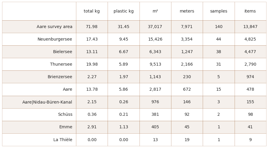
agg_caption = F"""
*__Below:__ The cumulative weights and measures for the {this_feature["name"]} and water bodies.*
"""
md(agg_caption)

Below: The cumulative weights and measures for the Aare survey area and water bodies.

# make table
data = dims_table.reset_index()
colLabels = data.columns

fig, ax = plt.subplots(figsize=(len(colLabels)*1.8,len(data)*.7))
sut.hide_spines_ticks_grids(ax)

table_one = sut.make_a_table(ax, data.values, colLabels=colLabels, colWidths=[.28, *[.12]*6], a_color=a_color)
table_one.get_celld()[(0,0)].get_text().set_text(" ")

plt.tight_layout()
plt.show()

3.1.3. Distribution of survey results¶

# the surveys to chart
fd_dindex = dt_all.set_index("date")

# all the other surveys
ots = dict(level_to_exclude=this_feature["level"], components_to_exclude=fd[this_feature["level"]].unique())
dts_date = sut.the_other_surveys(a_data, **ots)
dts_date.head()

# the survey totals from all other survey areas
dts_date = dts_date.groupby(["loc_date","date"], as_index=False)[unit_label].sum()
dts_date.set_index("date", inplace=True)

# get the monthly or quarterly results for the feature
resample_plot, rate = sut.quarterly_or_monthly_values(fd_dindex , this_feature["name"], vals=unit_label, quarterly=["ticino"])

# scale the chart as needed to accomodate for extreme values
y_lim = 95
y_limit = np.percentile(dts_date[unit_label], y_lim)

# label for the chart that alerts to the scale
not_included = F"Values greater than {round(y_limit, 1)} not shown."

# figure caption
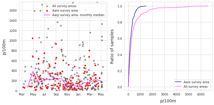
chart_notes = F"""
*__Left:__ {this_feature["name"]}, {start_date[:7]} through {end_date[:7]}, n={t["loc_date"]}. {not_included} __Right:__ {this_feature["name"]} empirical cumulative distribution of survey results.*
"""
md(chart_notes )

Left: Aare survey area, 2020-03 through 2021-05, n=140. Values greater than 1766.2 not shown. Right: Aare survey area empirical cumulative distribution of survey results.

# months locator, can be confusing
# https://matplotlib.org/stable/api/dates_api.html
months = mdates.MonthLocator(interval=1)
months_fmt = mdates.DateFormatter("%b")
days = mdates.DayLocator(interval=7)

fig, axs = plt.subplots(1,2, figsize=(10,5))

# the survey totals by day
ax = axs[0]

# feature surveys
sns.scatterplot(data=dts_date, x=dts_date.index, y=unit_label, label=top, color="black", alpha=0.4,  ax=ax)
# all other surveys
sns.scatterplot(data=fd_dindex, x=fd_dindex.index, y=unit_label, label=this_feature["name"], color="red", s=34, ec="white", ax=ax)

# monthly or quaterly plot
sns.lineplot(data=resample_plot, x=resample_plot.index, y=resample_plot, label=F"{this_feature['name']}: {rate} median", color="magenta", ax=ax)

ax.set_ylim(0,y_limit )
ax.set_ylabel(unit_label, **ck.xlab_k14)

ax.set_xlabel("")
ax.xaxis.set_minor_locator(days)
ax.xaxis.set_major_formatter(months_fmt)
ax.legend()

# the cumlative distributions:
axtwo = axs[1]

# the feature of interest
feature_ecd = ECDF(dt_all[unit_label].values)    
sns.lineplot(x=feature_ecd.x, y=feature_ecd.y, color="darkblue", ax=axtwo, label=this_feature["name"])

# the other features
other_features = ECDF(dts_date[unit_label].values)
sns.lineplot(x=other_features.x, y=other_features.y, color="magenta", label=top, linewidth=1, ax=axtwo)

axtwo.set_xlabel(unit_label, **ck.xlab_k14)
axtwo.set_ylabel("Ratio of samples", **ck.xlab_k14)

plt.tight_layout()
plt.show()

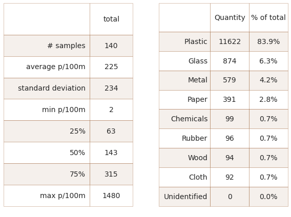
3.1.4. Summary data and material types¶

Left: Aare survey area summary of survey totals. Right: Aare survey area material type and percent of total.

# get the basic statistics from pd.describe
cs = dt_all[unit_label].describe().round(2)

# change the names
csx = sut.change_series_index_labels(cs, sut.create_summary_table_index(unit_label, lang="EN"))

combined_summary = sut.fmt_combined_summary(csx, nf=[])

fd_mat_totals = sut.fmt_pct_of_total(fd_mat_totals)
fd_mat_totals = sut.make_string_format(fd_mat_totals)

# applly new column names for printing
cols_to_use = {"material":"Material","quantity":"Quantity", "% of total":"% of total"}
fd_mat_t = fd_mat_totals[cols_to_use.keys()].values

# make tables
fig, axs = plt.subplots(1,2, figsize=(8,6))

# summary table
# names for the table columns
a_col = [this_feature["name"], "total"]

axone = axs[0]
sut.hide_spines_ticks_grids(axone)

table_two = sut.make_a_table(axone, combined_summary,  colLabels=a_col, colWidths=[.5,.25,.25],  bbox=[0,0,1,1], **{"loc":"lower center"})
table_two.get_celld()[(0,0)].get_text().set_text(" ")
table_two.set_fontsize(14)

# material table
axtwo = axs[1]
axtwo.set_xlabel(" ")
sut.hide_spines_ticks_grids(axtwo)

table_three = sut.make_a_table(axtwo, fd_mat_t,  colLabels=list(cols_to_use.values()), colWidths=[.4, .3,.3],  bbox=[0,0,1,1], **{"loc":"lower center"})
table_three.get_celld()[(0,0)].get_text().set_text(" ")

plt.tight_layout()
plt.subplots_adjust(wspace=0.2)
plt.show()

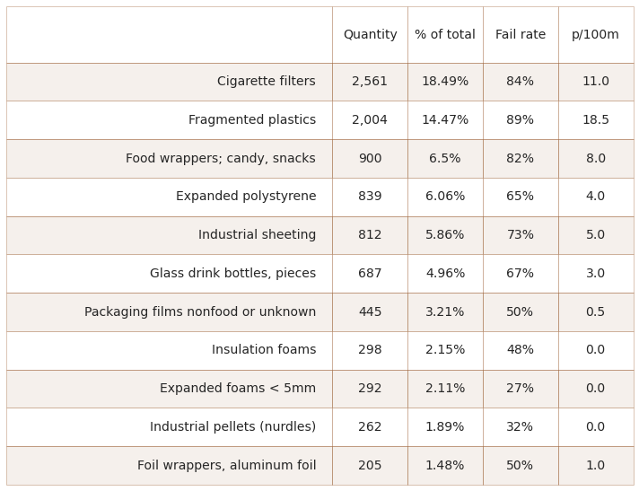
3.2. The most common objects¶

The most common objects are the ten most abundant by quantity AND/OR objects identified in at least 50% of all surveys.

# the top ten by quantity
most_abundant = code_totals.sort_values(by="quantity", ascending=False)[:10]

# the most common
most_common = code_totals[code_totals["fail rate"] >= a_fail_rate].sort_values(by="quantity", ascending=False)

# merge with most_common and drop duplicates
m_common = pd.concat([most_abundant, most_common]).drop_duplicates()

# get percent of total
m_common_percent_of_total = m_common.quantity.sum()/code_totals.quantity.sum()

# figure caption
rb_string = F"""
*__Below:__ {this_feature['name']} most common objects: fail rate >/= {a_fail_rate}%  and/or top ten by quantity. Combined, the most abundant objects represent {int(m_common_percent_of_total*100)}% of all objects found.*

Note : {unit_label} = median survey value.
"""
md(rb_string)

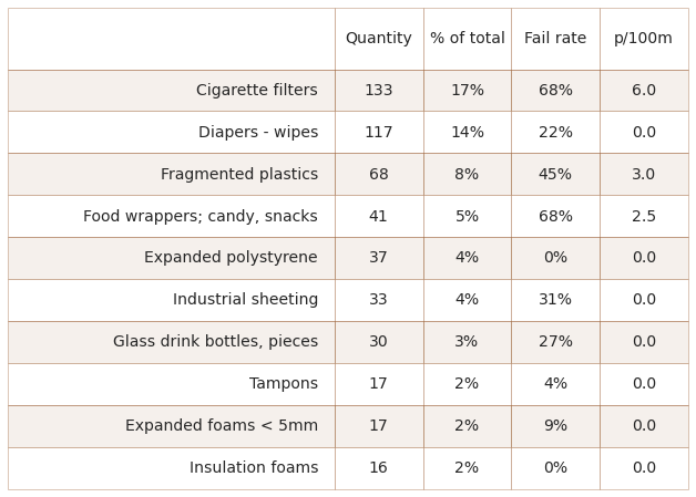
Below: Aare survey area most common objects: fail rate >/= 50% and/or top ten by quantity. Combined, the most abundant objects represent 67% of all objects found.

Note : p/100m = median survey value.

# format values for table
m_common["item"] = m_common.index.map(lambda x: code_description_map.loc[x])
m_common["% of total"] = m_common["% of total"].map(lambda x: F"{x}%")
m_common["quantity"] = m_common.quantity.map(lambda x: "{:,}".format(x))
m_common["fail rate"] = m_common["fail rate"].map(lambda x: F"{x}%")
m_common[unit_label] = m_common[unit_label].map(lambda x: F"{round(x,1)}")

cols_to_use = {"item":"Item","quantity":"Quantity", "% of total":"% of total", "fail rate":"Fail rate", unit_label:unit_label}
all_survey_areas = m_common[cols_to_use.keys()].values

fig, axs = plt.subplots(figsize=(10,len(m_common)*.7))

sut.hide_spines_ticks_grids(axs)

table_four = sut.make_a_table(axs, all_survey_areas,  colLabels=list(cols_to_use.values()), colWidths=[.52, .12,.12,.12, .12],  bbox=[0,0,1,1], **{"loc":"lower center"})
table_four.get_celld()[(0,0)].get_text().set_text(" ")
table_four.set_fontsize(14)
plt.tight_layout()
plt.show()

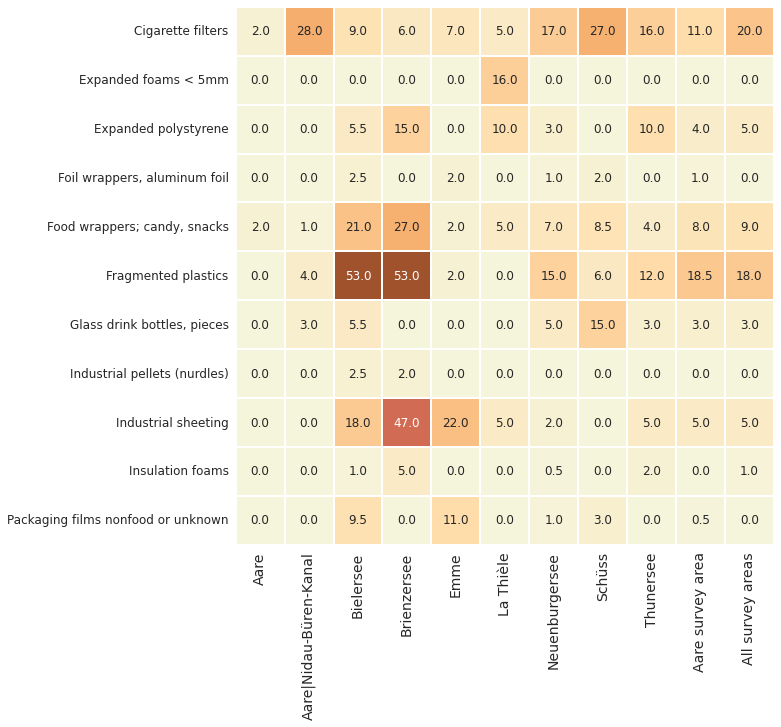
3.2.1. Most common objects by water feature¶

Below: Aare survey area most common objects: median p/100m

# aggregated survey totals for the most common codes for all the water features
m_common_st = fd[fd.code.isin(m_common.index)].groupby([this_level, "loc_date","code"], as_index=False).agg(agg_pcs_quantity)
m_common_ft = m_common_st.groupby([this_level, "code"], as_index=False)[unit_label].median()

# proper name of water feature for display
m_common_ft["f_name"] = m_common_ft[this_level].map(lambda x: comp_labels[x])

# map the desctiption to the code
m_common_ft["item"] = m_common_ft.code.map(lambda x: code_description_map.loc[x])

# pivot that
m_c_p = m_common_ft[["item", unit_label, "f_name"]].pivot(columns="f_name", index="item")

# quash the hierarchal column index
m_c_p.columns = m_c_p.columns.get_level_values(1)

# the aggregated totals for the survey area

c = sut.aggregate_to_group_name(fd[fd.code.isin(m_common.index)], column="code", name=this_feature["name"], val="med")

m_c_p[this_feature["name"]]= sut.change_series_index_labels(c, {x:code_description_map.loc[x] for x in c.index})

# the aggregated totals of all the data
c = sut.aggregate_to_group_name(a_data[(a_data.code.isin(m_common.index))], column="code", name=top, val="med")
m_c_p[top] = sut.change_series_index_labels(c, {x:code_description_map.loc[x] for x in c.index})

# chart that
fig, ax  = plt.subplots(figsize=(len(m_c_p.columns)*.9,len(m_c_p)*.9))
axone = ax

sns.heatmap(m_c_p, ax=axone, cmap=cmap2, annot=True, annot_kws={"fontsize":12}, fmt=".1f", square=True, cbar=False, linewidth=.1, linecolor="white")
axone.set_xlabel("")
axone.set_ylabel("")
axone.tick_params(labelsize=14, which="both", axis="x")
axone.tick_params(labelsize=12, which="both", axis="y")

plt.setp(axone.get_xticklabels(), rotation=90)

plt.show()

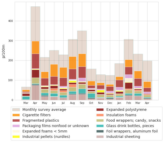
3.2.2. Most common objects monthly average¶

# collect the survey results of the most common objects
m_common_m = fd[(fd.code.isin(m_common.index))].groupby(["loc_date","date","code", "groupname"], as_index=False).agg(agg_pcs_quantity)
m_common_m.set_index("date", inplace=True)

# set the order of the chart, group the codes by groupname columns
an_order = m_common_m.groupby(["code","groupname"], as_index=False).quantity.sum().sort_values(by="groupname")["code"].values

# a manager dict for the monthly results of each code
mgr = {}

# get the monhtly results for each code:
for a_group in an_order:
    # resample by month
    a_plot = m_common_m[(m_common_m.code==a_group)][unit_label].resample("M").mean().fillna(0)
    this_group = {a_group:a_plot}
    mgr.update(this_group)

monthly_mc = F"""
*__Below:__ {this_feature["name"]}, monthly average survey result {unit_label}, with detail of the most common objects.*
"""
md(monthly_mc)

Below: Aare survey area, monthly average survey result p/100m, with detail of the most common objects.

months={
    0:"Jan",
    1:"Feb",
    2:"Mar",
    3:"Apr",
    4:"May",
    5:"Jun",
    6:"Jul",
    7:"Aug",
    8:"Sep",
    9:"Oct",
    10:"Nov",
    11:"Dec"
}

# convenience function to lable x axis
def new_month(x):
    if x <= 11:
        this_month = x
    else:
        this_month=x-12    
    return this_month

fig, ax = plt.subplots(figsize=(10,7))

# define a bottom
bottom = [0]*len(mgr["G27"])

# the monhtly survey average for all objects and locations
monthly_fd = fd.groupby(["loc_date", "date"], as_index=False).agg(agg_pcs_quantity)
monthly_fd.set_index("date", inplace=True)
m_fd = monthly_fd[unit_label].resample("M").mean().fillna(0)

# define the xaxis
this_x = [i for i,x in  enumerate(m_fd.index)]

# plot the monthly total survey average
ax.bar(this_x, m_fd.to_numpy(), color=a_color, alpha=0.2, linewidth=1, edgecolor="teal", width=1, label="Monthly survey average") 

# plot the monthly survey average of the most common objects
for i, a_group in enumerate(an_order): 
    
    # define the axis
    this_x = [i for i,x in  enumerate(mgr[a_group].index)]
    
    # collect the month
    this_month = [x.month for i,x in enumerate(mgr[a_group].index)]
    
    # if i == 0 laydown the first bars
    if i == 0:
        ax.bar(this_x, mgr[a_group].to_numpy(), label=a_group, color=colors_palette[a_group], linewidth=1, alpha=0.6 ) 
    # else use the previous results to define the bottom
    else:
        bottom += mgr[an_order[i-1]].to_numpy()        
        ax.bar(this_x, mgr[a_group].to_numpy(), bottom=bottom, label=a_group, color=colors_palette[a_group], linewidth=1, alpha=0.8)
        
# collect the handles and labels from the legend
handles, labels = ax.get_legend_handles_labels()

# set the location of the x ticks
ax.xaxis.set_major_locator(ticker.FixedLocator([i for i in np.arange(len(this_x))]))
ax.set_ylabel(unit_label, **ck.xlab_k14)

# label the xticks by month
axisticks = ax.get_xticks()
labelsx = [months[new_month(x-1)] for x in  this_month]
plt.xticks(ticks=axisticks, labels=labelsx)

# make the legend
# swap out codes for descriptions
new_labels = [code_description_map.loc[x] for x in labels[1:]]
new_labels = new_labels[::-1]

# insert a label for the monthly average
new_labels.insert(0,"Monthly survey average")
handles = [handles[0], *handles[1:][::-1]]
    
plt.legend(handles=handles, labels=new_labels, bbox_to_anchor=(.5, -.05), loc="upper center",  ncol=2, fontsize=14)       
plt.show()

3.3. Survey results and land use¶

The land use mix is a unique representation of the type and amplitude of the economic activity and the environmental conditions around the survey location. The key indicators from the survey results are compared against the land use rates for a radius of 1500m from the survey location.

An association is a relationship between the survey results and the land use profile that is unlikely due to chance. The magnitude of the relationship is neither defined nor linear.

Ranked correlation is a non-parametric test to determine if there is a statistically significant relationship between land use and the objects identified in a litter survey.

The method used is the Spearman’s rho or Spearmans ranked correlation coefficient. The test results are evaluated at p<0.05 for all valid lake samples in the survey area.

Red/rose is a positive association
Yellow is a negative association
White means that p>0.05, there is no statistical basis to assume an association

corr_data = fd[(fd.code.isin(m_common.index))&(fd.water_name_slug.isin(lakes_of_interest))].copy()

alert_less_than_100 = len(corr_data.loc_date.unique()) <= 100

if alert_less_than_100:
    warning = F"""**There are less than 100 samples, proceed with caution. Beach litter surveys have alot of variance**"""
else:
    warning = ""

association = F"""*__Below:__ {this_feature["name"]} ranked correlation of the most common objects with respect to land use profile.
For all valid lake samples n={len(corr_data.loc_date.unique())}.*

{warning}
"""
md(association)

Below: Aare survey area ranked correlation of the most common objects with respect to land use profile. For all valid lake samples n=118.

# chart the results of test for association
fig, axs = plt.subplots(len(m_common.index),len(luse_exp), figsize=(len(luse_exp)+7,len(m_common.index)+1), sharey="row")

# the test is conducted on the survey results for each code
for i,code in enumerate(m_common.index):
    # slice the data
    data = corr_data[corr_data.code == code]
    
    # run the test on for each land use feature
    for j, n in enumerate(luse_exp):       
        # assign ax and set some parameters
        ax=axs[i, j]
        ax.grid(False)
        ax.tick_params(axis="both", which="both",bottom=False,top=False,labelbottom=False, labelleft=False, left=False)
        
        # check the axis and set titles and labels       
        if i == 0:
            ax.set_title(F"{n}")
        else:
            pass
        
        if j == 0:
            ax.set_ylabel(F"{code_description_map[code]}", rotation=0, ha="right", **ck.xlab_k14)
            ax.set_xlabel(" ")
        else:
            ax.set_xlabel(" ")
            ax.set_ylabel(" ")
        # run test
        _, corr, a_p = sut.make_plot_with_spearmans(data, ax, n)
        
        # if siginficant set adjust color to direction
        if a_p < 0.05:
            if corr > 0:
                ax.patch.set_facecolor("salmon")
                ax.patch.set_alpha(0.5)
            else:
                ax.patch.set_facecolor("palegoldenrod")
                ax.patch.set_alpha(0.5)

plt.tight_layout()
plt.subplots_adjust(wspace=0, hspace=0)
plt.show()

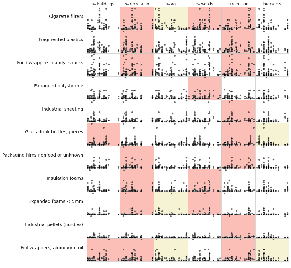
Key: if p>0.05 = white, if p < 0.05 and \(\rho\) > 0 = red, if p < 0.05 and \(\rho\) < 0 = yellow

3.4. Utility of the objects found¶

The utility type is based on the utilization of the object prior to it being discarded or object description if the original use is undetermined. Identified objects are classified into one of 260 predefined categories. The categories are grouped according to utilization or item description.

wastewater: items released from water treatment plants includes items likely toilet flushed
micro plastics (< 5mm): fragmented plastics and pre-production plastic resins
infrastructure: items related to construction and maintenance of buildings, roads and water/power supplies
food and drink: all materials related to consuming food and drink
agriculture: primarily industrial sheeting i.e., mulch and row covers, greenhouses, soil fumigation, bale wraps. Includes hard plastics for agricultural fencing, flowerpots etc.
tobacco: primarily cigarette filters, includes all smoking related material
recreation: objects related to sports and leisure i.e., fishing, hunting, hiking etc.
packaging non food and drink: packaging material not identified as food, drink nor tobacco related
plastic fragments: plastic pieces of undetermined origin or use
personal items: accessories, hygiene and clothing related

See the annex for the complete list of objects identified, includes descriptions and group classification. The section Code groups describes each code group in detail and provides a comprehensive list of all objects in a group.

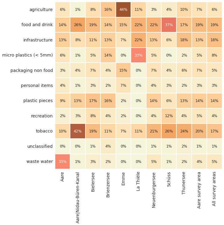
Below: Aare survey area utility of objects found % of total by water feature. Fragmented objects with no clear identification remain classified by size.

# code groups resluts aggregated by survey
groups = ["loc_date","groupname"]
cg_t = fd.groupby([this_level,*groups], as_index=False).agg(agg_pcs_quantity)

# the total per water feature
cg_tq = cg_t.groupby(this_level).quantity.sum()

# get the fail rates for each group per survey
cg_t["fail"]=False
cg_t["fail"] = cg_t.quantity.where(lambda x: x == 0, True)

# aggregate all that for each municipality
agg_this = {unit_label:"median", "quantity":"sum", "fail":"sum", "loc_date":"nunique"} 
cg_t = cg_t.groupby([this_level, "groupname"], as_index=False).agg(agg_this)

# assign survey area total to each record
for a_feature in cg_tq.index:
    cg_t.loc[cg_t[this_level] == a_feature, "f_total"] = cg_tq.loc[a_feature]

# get the percent of total for each group for each survey area
cg_t["pt"] = (cg_t.quantity/cg_t.f_total).round(2)

# pivot that
data_table = cg_t.pivot(columns=this_level, index="groupname", values="pt")

# repeat for the survey area
data_table[bassin_label] = sut.aggregate_to_group_name(fd, unit_label=unit_label, column="groupname", name=bassin_label, val="pt")

# repeat for all the data
data_table[top] = sut.aggregate_to_group_name(a_data, unit_label=unit_label, column="groupname", name=top, val="pt")

data = data_table
data.rename(columns={x:wname_wname.loc[x][0] for x in data.columns[:-2]}, inplace=True)

fig, ax = plt.subplots(figsize=(10,10))

axone = ax
sns.heatmap(data , ax=axone, cmap=cmap2, annot=True, annot_kws={"fontsize":12}, cbar=False, fmt=".0%", linewidth=.1, square=True, linecolor="white")

axone.set_ylabel("")
axone.set_xlabel("")
axone.tick_params(labelsize=14, which="both", axis="both", labeltop=False, labelbottom=True)

plt.setp(axone.get_xticklabels(), rotation=90, fontsize=14)
plt.setp(axone.get_yticklabels(), rotation=0, fontsize=14)

plt.show()

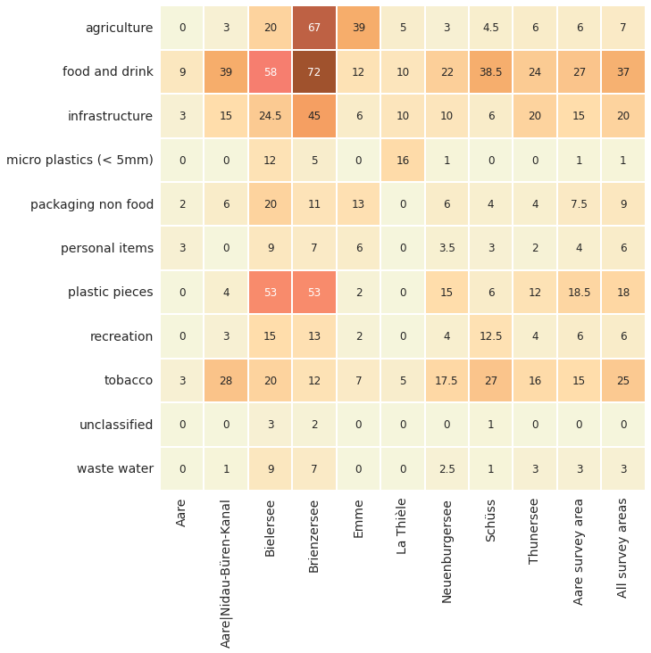
cg_medpcm = F"""
<br></br>
*__Below:__ {this_feature["name"]} utility of objects found median {unit_label}. Fragmented objects with no clear identification remain classified by size.*
"""
md(cg_medpcm)

Below: Aare survey area utility of objects found median p/100m. Fragmented objects with no clear identification remain classified by size.

# median p/50m of all the water features
data_table = cg_t.pivot(columns="water_name_slug", index="groupname", values=unit_label)

# the survey area columns
data_table[bassin_label] = sut.aggregate_to_group_name(fd, unit_label=unit_label, column="groupname", name=bassin_label, val="med")

# column for all the surveys
data_table[top] = sut.aggregate_to_group_name(a_data, unit_label=unit_label, column="groupname", name=top, val="med")

# merge with data_table
data = data_table
data.rename(columns={x:wname_wname.loc[x][0] for x in data.columns[:-2]}, inplace=True)
fig, ax = plt.subplots(figsize=(10,10))

axone = ax
sns.heatmap(data , ax=axone, cmap=cmap2, annot=True, annot_kws={"fontsize":12}, fmt="g", cbar=False, linewidth=.1, square=True, linecolor="white")

axone.set_xlabel("")
axone.set_ylabel("")
axone.tick_params(labelsize=14, which="both", axis="both", labeltop=False, labelbottom=True)

plt.setp(axone.get_xticklabels(), rotation=90, fontsize=14)
plt.setp(axone.get_yticklabels(), rotation=0, fontsize=14)

plt.show()

3.5. Rivers¶

rivers = fd[fd.w_t == "r"].copy()
r_smps = rivers.groupby(["loc_date", "date", "location", "water_name_slug"], as_index=False).agg(agg_pcs_quantity)
l_smps = fd[fd.w_t == "l"].groupby(["loc_date","date","location", "water_name_slug"], as_index=False).agg(agg_pcs_quantity)

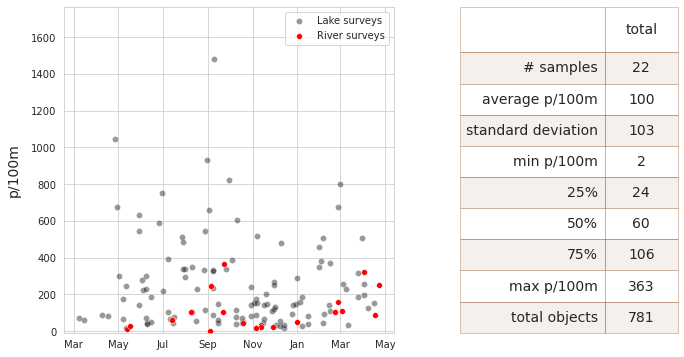
chart_notes = F"""
*__Left:__ {this_feature["name"]} rivers, {start_date[:7]} through {end_date[:7]}, n={len(r_smps.loc_date.unique())}. {not_included} __Right:__ Summary data.*
"""
md(chart_notes )

Left: Aare survey area rivers, 2020-03 through 2021-05, n=22. Values greater than 1766.2 not shown. Right: Summary data.

cs = r_smps[unit_label].describe().round(2)

# add project totals
cs["total objects"] = r_smps.quantity.sum()

# change the names
csx = sut.change_series_index_labels(cs, sut.create_summary_table_index(unit_label, lang="EN"))

combined_summary = sut.fmt_combined_summary(csx, nf=[])

# make the charts
fig = plt.figure(figsize=(11,6))

aspec = fig.add_gridspec(ncols=11, nrows=3)

ax = fig.add_subplot(aspec[:, :6])

line_label = F"{rate} median:{top}"

sns.scatterplot(data=l_smps, x="date", y=unit_label, color="black", alpha=0.4, label="Lake surveys", ax=ax)
sns.scatterplot(data=r_smps, x="date", y=unit_label, color="red", s=34, ec="white",label="River surveys", ax=ax)

ax.set_ylim(-10,y_limit )

ax.set_xlabel("")
ax.set_ylabel(unit_label, **ck.xlab_k14)

ax.xaxis.set_minor_locator(days)
ax.xaxis.set_major_formatter(months_fmt)

a_col = [this_feature["name"], "total"]

axone = fig.add_subplot(aspec[:, 7:])
sut.hide_spines_ticks_grids(axone)

table_five = sut.make_a_table(axone, combined_summary,  colLabels=a_col, colWidths=[.5,.25,.25],  bbox=[0,0,1,1], **{"loc":"lower center"})
table_five.get_celld()[(0,0)].get_text().set_text(" ")


plt.show()

3.5.1. Rivers most common objects¶

riv_mcommon = F"""
*__Below:__ {this_feature["name"]} rivers, most common objects {unit_label}: median survey value*
"""
md(riv_mcommon)

Below: Aare survey area rivers, most common objects p/100m: median survey value

# the most common items rivers
r_codes = rivers.groupby("code").agg({"quantity":"sum", "fail":"sum", unit_label:"median"})
r_codes["Fail rate"] = (r_codes.fail/r_smps.loc_date.nunique()*100).astype("int")

# top ten
r_byq = r_codes.sort_values(by="quantity", ascending=False)[:10].index

# most common
r_byfail = r_codes[r_codes["Fail rate"] > 49.99].index
r_most_common = list(set(r_byq) | set(r_byfail))

# format for display
r_mc= r_codes.loc[r_most_common].copy()
r_mc["item"] = r_mc.index.map(lambda x: code_description_map.loc[x])
r_mc.sort_values(by="quantity", ascending=False, inplace=True)

r_mc["% of total"]=((r_mc.quantity/r_codes.quantity.sum())*100).astype("int")
r_mc["% of total"] = r_mc["% of total"].map(lambda x: F"{x}%")
r_mc["quantity"] = r_mc.quantity.map(lambda x: "{:,}".format(x))
r_mc["Fail rate"] = r_mc["Fail rate"].map(lambda x: F"{x}%")
r_mc["p/50m"] = r_mc[unit_label].map(lambda x: F"{np.ceil(x)}")
r_mc.rename(columns=cols_to_use, inplace=True)

data=r_mc[["Item","Quantity", "% of total", "Fail rate", unit_label]]

fig, axs = plt.subplots(figsize=(11,len(data)*.8))

sut.hide_spines_ticks_grids(axs)

table_six = sut.make_a_table(axs, data.values,  colLabels=list(data.columns), colWidths=[.48, .13,.13,.13, .13], **{"loc":"lower center"})
table_six.get_celld()[(0,0)].get_text().set_text(" ")


plt.show()
plt.tight_layout()
plt.close()

3.6. Annex¶

3.6.1. Fragmented foams and plastics by size¶

The table below contains the “Gfoam” and “Gfrags” components grouped for analysis. Objects labeled expanded foams are grouped as Gfoam and includes all expanded polystyrene foamed plastics > 0.5 cm. Plastic pieces and objects made of combined plastic and foamed plastic materials > 0.5 cm. are grouped for analysis as Gfrags.

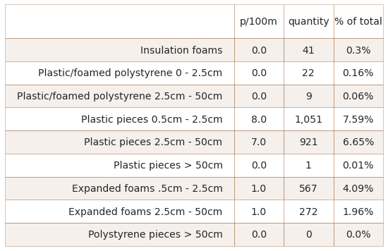
Below: Aare survey area fragmented foams and plastics by size group.

# collect the data before aggregating foams for all locations in the survye area
# group by loc_date and code
# Combine the different sizes of fragmented plastics and styrofoam
# the codes for the foams
some_foams = ["G81", "G82", "G83", "G74"]

# the codes for the fragmented plastics
some_frag_plas = list(before_agg[before_agg.groupname == "plastic pieces"].code.unique())

fd_frags_foams = before_agg[(before_agg.code.isin([*some_frag_plas, *some_foams]))&(before_agg.location.isin(t["locations"]))].groupby(["loc_date","code"], as_index=False).agg(agg_pcs_quantity)
fd_frags_foams = fd_frags_foams.groupby("code").agg(agg_pcs_median)

# add code description and format for printing
fd_frags_foams["item"] = fd_frags_foams.index.map(lambda x: code_description_map.loc[x])
fd_frags_foams["% of total"] = (fd_frags_foams.quantity/fd.quantity.sum()*100).round(2)
fd_frags_foams["% of total"] = fd_frags_foams["% of total"].map(lambda x: F"{x}%")
fd_frags_foams["quantity"] = fd_frags_foams["quantity"].map(lambda x: F"{x:,}")

# table data
data = fd_frags_foams[["item",unit_label, "quantity", "% of total"]]

fig, axs = plt.subplots(figsize=(len(data.columns)*2.4,len(data)*.7))

sut.hide_spines_ticks_grids(axs)

table_seven = sut.make_a_table(axs,data.values,  colLabels=data.columns, colWidths=[.6, .13, .13, .13], a_color=a_color)
table_seven.get_celld()[(0,0)].get_text().set_text(" ")
table_seven.set_fontsize(14)

plt.show()
plt.tight_layout()
plt.close()

3.6.2. The survey locations¶

# display the survey locations
disp_columns = ["latitude", "longitude", "city"]
disp_beaches = dfBeaches.loc[t["locations"]][disp_columns]
disp_beaches.reset_index(inplace=True)
disp_beaches.rename(columns={"slug":"location"}, inplace=True)
disp_beaches.set_index("location", inplace=True, drop=True)

disp_beaches

	latitude	longitude	city
location
aare-port	47.116170	7.269550	Port
schutzenmatte	47.057666	7.634001	Burgdorf
la-petite-plage	46.785054	6.656877	Yverdon-les-Bains
weissenau-neuhaus	46.676583	7.817528	Unterseen
evole-plage	46.989477	6.923920	Neuchâtel
oberi-chlihochstetten	46.896025	7.532114	Rubigen
plage-de-serriere	46.984850	6.913450	Neuchâtel
mullermatte	47.133339	7.227907	Biel/Bienne
bielersee_vinelz_fankhausers	47.038398	7.108311	Vinelz
erlach-camping-strand	47.047159	7.097854	Erlach
gummligrabbe	46.989290	7.250730	Kallnach
mannewil	46.996382	7.239024	Kallnach
schusspark-strand	47.146500	7.268620	Biel/Bienne
plage-de-cheyres	46.818689	6.782256	Cheyres-Châbles
thun-strandbad	46.739939	7.633520	Thun
oben-am-see	46.744451	8.049921	Brienz (BE)
thunersee_spiez_meierd_1	46.704437	7.657882	Spiez
spackmatt	47.223749	7.576711	Luterbach
luscherz-plage	47.047955	7.151242	Lüscherz
strandboden-biel	47.132510	7.233142	Biel/Bienne
signalpain	46.786200	6.647360	Yverdon-les-Bains
pointe-dareuse	46.946190	6.870970	Boudry
nidau-strand	47.127196	7.232613	Nidau
camp-des-peches	47.052812	7.074053	Le Landeron
delta-park	46.720078	7.635304	Spiez
pecos-plage	46.803590	6.636650	Grandson
beich	47.048495	7.200528	Walperswil
aare_suhrespitz_badert	47.405669	8.066018	Aarau
sundbach-strand	46.684386	7.794768	Beatenberg
wycheley	46.740370	8.048640	Brienz (BE)
aare_koniz_hoppej	46.934588	7.458170	Köniz
camping-gwatt-strand	46.727140	7.629620	Thun
bern-tiergarten	46.933157	7.452004	Bern
la-thiele_le-mujon_confluence	46.775340	6.630900	Yverdon-les-Bains
nouvelle-plage	46.856646	6.848428	Estavayer
augustmutzenbergstrandweg	46.686640	7.689760	Spiez
aare_bern_gerberm	46.989363	7.452098	Bern
brugg-be-buren-bsg-standort	47.122220	7.281410	Brügg
ruisseau-de-la-croix-plage	46.813920	6.774700	Cheyres-Châbles
ligerz-strand	47.083979	7.135894	Ligerz
hafeli	46.690283	7.898592	Bönigen
aare-solothurn-lido-strand	47.196949	7.521643	Solothurn
bern-fahrstrasse	46.975866	7.444210	Bern
gals-reserve	47.046272	7.085007	Gals
hauterive-petite-plage	47.010797	6.980304	Hauterive (NE)
aare-limmatspitz	47.501060	8.237371	Gebenstorf
aare_brugg_buchie	47.494855	8.236558	Brugg
luscherz-two	47.047519	7.152829	Lüscherz
impromptu_cudrefin	46.964496	7.027936	Cudrefin
aare_post	47.116665	7.271953	Port
aare_bern_scheurerk	46.970967	7.452586	Bern

3.6.3. Inventory of items¶

pd.set_option("display.max_rows", None)
complete_inventory = code_totals[code_totals.quantity>0][["item", "groupname", "quantity", "% of total","fail rate"]]
complete_inventory.sort_values(by="quantity", ascending=False)

	item	groupname	quantity	% of total	fail rate
code
G27	Cigarette filters	tobacco	2561	18.49	84
Gfrags	Fragmented plastics	plastic pieces	2004	14.47	89
G30	Food wrappers; candy, snacks	food and drink	900	6.50	82
Gfoam	Expanded polystyrene	infrastructure	839	6.06	65
G67	Industrial sheeting	agriculture	812	5.86	73
G200	Glass drink bottles, pieces	food and drink	687	4.96	67
G941	Packaging films nonfood or unknown	packaging non food	445	3.21	50
G74	Insulation foams	infrastructure	298	2.15	48
G117	Expanded foams < 5mm	micro plastics (< 5mm)	292	2.11	27
G112	Industrial pellets (nurdles)	micro plastics (< 5mm)	262	1.89	32
G98	Diapers - wipes	waste water	258	1.86	28
G89	Plastic construction waste	infrastructure	219	1.58	49
G177	Foil wrappers, aluminum foil	food and drink	205	1.48	50
G95	Cotton bud/swab sticks	waste water	201	1.45	49
G25	Tobacco; plastic packaging, containers	tobacco	159	1.15	43
G904	Plastic fireworks	recreation	155	1.12	41
G156	Paper fragments	packaging non food	150	1.08	28
G178	Metal bottle caps and lids	food and drink	123	0.89	40
G106	Plastic fragments angular <5mm	micro plastics (< 5mm)	104	0.75	27
G940	Foamed EVA for crafts and sports	recreation	102	0.74	11
G21	Drink lids	food and drink	98	0.71	31
G213	Paraffin wax	recreation	98	0.71	18
G50	String < 1cm	recreation	96	0.69	36
G23	Lids unidentified	packaging non food	93	0.67	30
G33	Lids for togo drinks plastic	food and drink	87	0.63	35
G922	Labels, bar codes	packaging non food	87	0.63	32
G35	Straws and stirrers	food and drink	82	0.59	35
G186	Industrial scrap	infrastructure	82	0.59	20
G24	Plastic lid rings	food and drink	80	0.58	28
G10	Food containers single use foamed or plastic	food and drink	74	0.53	28
G211	Swabs, bandaging, medical	personal items	73	0.53	32
G31	Lollypop sticks	food and drink	71	0.51	30
G32	Toys and party favors	recreation	67	0.48	32
G923	Tissue, toilet paper, napkins, paper towels	personal items	62	0.45	24
G73	Foamed items & pieces (non packaging/insulatio...	recreation	58	0.42	19
G66	Straps/bands; hard, plastic package fastener	infrastructure	55	0.40	30
G153	Cups, food containers, wrappers (paper)	food and drink	54	0.39	17
G203	Tableware ceramic or glass, cups, plates, pieces	food and drink	49	0.35	13
G22	Lids for chemicals, detergents (non-food)	infrastructure	49	0.35	18
G936	Sheeting ag. greenhouse film	agriculture	48	0.35	13
G908	Tape; electrical, insulating	infrastructure	46	0.33	20
G93	Cable ties; steggel, zip, zap straps	infrastructure	45	0.32	17
G204	Bricks, pipes not plastic	infrastructure	45	0.32	10
G152	Cigarette boxes, tobacco related paper/cardboard	tobacco	43	0.31	13
G3	Plastic bags, carier bags	packaging non food	42	0.30	17
G191	Wire and mesh	agriculture	41	0.30	15
G96	Sanitary-pads/tampons, applicators	waste water	40	0.29	15
G100	Medical; containers/tubes/ packaging	waste water	40	0.29	22
G87	Tape, masking/duct/packing	infrastructure	39	0.28	18
G125	Balloons and balloon sticks	recreation	38	0.27	17
G91	Biomass holder	waste water	37	0.27	16
G905	Hair clip, hair ties, personal accessories pl...	personal items	35	0.25	19
G137	Clothing, towels & rags	personal items	35	0.25	10
G944	Pellet mass from injection molding	unclassified	34	0.25	2
G175	Cans, beverage	food and drink	31	0.22	13
G70	Shotgun cartridges	recreation	30	0.22	15
G927	String trimmer line, used to cut grass, weeds,...	infrastructure	27	0.19	8
G201	Jars, includes pieces	food and drink	27	0.19	8
G928	Ribbons and bows	personal items	27	0.19	11
G198	Other metal pieces < 50cm	infrastructure	26	0.19	14
G208	Glass or ceramic fragments > 2.5 cm	unclassified	26	0.19	7
G165	Ice cream sticks, toothpicks, chopsticks	food and drink	25	0.18	13
G159	Corks	food and drink	25	0.18	12
G131	Rubber bands	personal items	24	0.17	12
G942	Plastic shavings from lathes, CNC machining	unclassified	24	0.17	9
G26	Cigarette lighters	tobacco	23	0.17	13
G210	Other glass/ceramic	unclassified	21	0.15	4
G914	Paperclips, clothespins, plastic utility items	personal items	20	0.14	8
G90	Plastic flower pots	agriculture	20	0.14	10
G48	Rope, synthetic	recreation	19	0.14	11
G4	Small plastic bags; freezer, zip-lock etc.	packaging non food	19	0.14	7
G149	Paper packaging	packaging non food	19	0.14	6
G28	Pens, lids, mechanical pencils etc.	personal items	19	0.14	9
G34	Cutlery, plates and trays	food and drink	18	0.13	10
G144	Tampons	waste water	18	0.13	1
G7	Drink bottles < = 0.5L	food and drink	18	0.13	9
G158	Other paper items	packaging non food	17	0.12	5
G148	Cardboard (boxes and fragments)	packaging non food	16	0.12	6
G134	Other rubber	unclassified	16	0.12	7
G943	Fencing agriculture, plastic	agriculture	15	0.11	2
G170	Wood (processed)	agriculture	15	0.11	7
G194	Cables, metal wire(s) often inside rubber or p...	infrastructure	15	0.11	8
G101	Dog feces bag	personal items	14	0.10	7
G142	Rope , string or nets	recreation	14	0.10	6
G161	Processed timber	agriculture	13	0.09	5
G59	Fishing line monofilament (angling)	recreation	13	0.09	7
G939	Flowers, plants plastic	personal items	12	0.09	5
G167	Matches or fireworks	recreation	12	0.09	2
G124	Other plastic or foam products	unclassified	11	0.08	5
G146	Paper, cardboard	packaging non food	11	0.08	2
G931	Tape-caution for barrier, police, construction...	infrastructure	11	0.08	4
G115	Foamed plastic <5mm	micro plastics (< 5mm)	10	0.07	5
G919	Nails, screws, bolts etc.	infrastructure	10	0.07	4
G901	Mask medical, synthetic	personal items	10	0.07	6
G933	Bags, cases for accessories; glasses, electron...	personal items	10	0.07	5
G65	Buckets	agriculture	9	0.06	2
G155	Fireworks paper tubes and fragments	recreation	9	0.06	6
G2	Bags	packaging non food	9	0.06	3
G921	Ceramic tile and pieces	infrastructure	9	0.06	6
G918	Safety pins, paper clips, small metal utility ...	personal items	9	0.06	5
G135	Clothes, footware, headware, gloves	personal items	9	0.06	5
G20	Caps and lids	packaging non food	8	0.06	5
G176	Cans, food	food and drink	8	0.06	4
G133	Condoms incl. packaging	waste water	8	0.06	5
G917	Terracotta balls	unclassified	8	0.06	4
G68	Fiberglass fragments	infrastructure	8	0.06	5
G118	Small industrial spheres <5mm	micro plastics (< 5mm)	7	0.05	2
G122	Plastic fragments ( >1mm)	micro plastics (< 5mm)	7	0.05	0
G925	Packets: desiccant/ moisture absorbers, plasti...	packaging non food	7	0.05	3
G929	Electronics and pieces; sensors, headsets etc.	personal items	6	0.04	3
G49	Rope > 1cm	recreation	6	0.04	2
G182	Fishing; hooks, weights, lures, sinkers etc.	recreation	6	0.04	3
G38	Coverings; plastic packaging, sheeting for pro...	unclassified	6	0.04	3
G938	Toothpicks, dental floss plastic	food and drink	6	0.04	4
G126	Balls	recreation	6	0.04	2
G36	Bags/sacks heavy duty plastic for 25 Kg or mor...	agriculture	5	0.04	2
G64	Fenders	unclassified	5	0.04	2
G141	Carpet	unclassified	5	0.04	2
G29	Combs, brushes and sunglasses	personal items	5	0.04	2
G71	Shoes sandals	personal items	4	0.03	2
G104	Plastic fragments subrounded <5mm	micro plastics (< 5mm)	4	0.03	2
G926	Chewing gum, often contains plastics	food and drink	4	0.03	2
G103	Plastic fragments rounded <5mm	micro plastics (< 5mm)	4	0.03	2
G8	Drink bottles > 0.5L	food and drink	4	0.03	2
G913	Pacifier	personal items	4	0.03	2
G930	Foam earplugs	personal items	4	0.03	2
G119	Sheetlike user plastic (>1mm)	micro plastics (< 5mm)	4	0.03	1
G11	Cosmetics for the beach, e.g. sunblock	recreation	4	0.03	2
G157	Paper	packaging non food	4	0.03	2
G197	Other metal	infrastructure	4	0.03	2
G37	Mesh bags	personal items	4	0.03	2
G145	Other textiles	personal items	4	0.03	2
G6	Bottles and containers, plastic non food/drink	packaging non food	3	0.02	0
G151	Cartons, Tetrapacks	food and drink	3	0.02	1
G945	Razor blades	personal items	3	0.02	2
G99	Syringes - needles	personal items	3	0.02	2
G143	Sails and canvas	recreation	3	0.02	2
G12	Cosmetics, non-beach use personal care containers	personal items	3	0.02	2
G102	Flip-flops	personal items	2	0.01	1
G154	Newspapers or magazines	personal items	2	0.01	1
G129	Inner tubes and rubber sheets	unclassified	2	0.01	1
G181	Tableware metal; cups, cutlery etc.	food and drink	2	0.01	1
G188	Other cans < 4 L	infrastructure	2	0.01	0
G195	Batteries - household	personal items	2	0.01	1
G202	Light bulbs	unclassified	2	0.01	1
G111	Spheruloid pellets < 5mm	micro plastics (< 5mm)	2	0.01	1
G174	Aerosol spray cans	infrastructure	2	0.01	1
G136	Shoes	personal items	2	0.01	1
G43	Tags fishing or industry (security tags, seals)	recreation	2	0.01	1
G915	Reflectors, plastic mobility items	personal items	2	0.01	0
G916	Pencils and pieces	personal items	2	0.01	1
G39	Gloves	personal items	2	0.01	0
G52	Nets and pieces	recreation	2	0.01	1
G53	Nets and pieces < 50cm	recreation	1	0.01	0
G17	Injection gun cartridge	infrastructure	1	0.01	0
G902	Mask medical, cloth	personal items	1	0.01	0
G900	Gloves latex personal protective equipment	personal items	1	0.01	0
G13	Bottles, containers, drums to transport, store...	agriculture	1	0.01	0
G150	Milk cartons, tetrapack	food and drink	1	0.01	0
G172	Other wood > 50cm	agriculture	1	0.01	0
G97	Toilet fresheners	waste water	1	0.01	0
G60	Light sticks	recreation	1	0.01	0
G84	CD or CD box	personal items	1	0.01	0
G61	Other fishing related	recreation	1	0.01	0
G171	Other wood < 50cm	agriculture	1	0.01	0
G14	Engine oil bottles	unclassified	1	0.01	0
G94	Table cloth	recreation	1	0.01	0
G903	Hand sanitizer containers & packets	personal items	1	0.01	0
G179	Disposable BBQs	food and drink	1	0.01	0
G934	Sandbag, plastic for flood, erosion control etc..	agriculture	1	0.01	0
G128	Tires and belts	unclassified	1	0.01	0
G138	Shoes and sandals	personal items	1	0.01	0
G5	Generic plastic bags	packaging non food	1	0.01	0
G190	Paint cans	infrastructure	1	0.01	0
G41	Glove industrial/professional	agriculture	1	0.01	0
G107	Cylindrical pellets < 5mm	micro plastics (< 5mm)	1	0.01	0
G214	Oil/tar	infrastructure	1	0.01	0
G114	Films <5mm	micro plastics (< 5mm)	1	0.01	0
G40	Gloves household/gardening	personal items	1	0.01	0

Aare

Contents