21. More and less since 2018¶

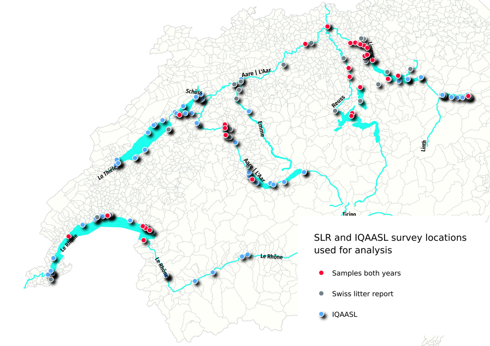
he first national beach litter report was produced in 2018. The Swiss Litter Report (SLR) was a project initiated by Gabriele Kuhl [Kuh] and supported by the World Wildlife Fund Switzerland [Fun]. The protocol was based on the Guide for monitoring marine litter [Han13], the project was managed by the WWF and the surveys were conducted by volunteers from both organizations. The project began in April 2017 and ended March 2018 the SLR covered much of the national territory except for the Ticino region.

The SLR collected 1,052 samples from 112 locations. More than 150 trained volunteers from 81 municipalities collected and categorized 98,474 pieces of trash from the shores of 48 lakes and 67 rivers in Switzerland. [Bla18]

The most obvious question is: Was there more or less litter observed in 2021 than 2018? To answer the question the survey locations from each project were first compared based on the land use profile within 1500m of each survey location for each project. The survey results were limited to:

Only objects that were identified in 2018 were considered

From this subset of data, the median survey total of all objects and the average survey total of the most common objects were compared to identify statistically significant changes in either direction from one project to the next. This test was conducted on two groups of the subset:

Rivers and lakes combined with samples from both projects
Only the lakes with samples from both projects

21.1. Scope of projects SLR - IQAASL¶

# make sure date is time stamp
survey_data["date"] = pd.to_datetime(survey_data["date"], format="%Y-%m-%d")

# get only the water features that were sampled in 2021
after_2020 = survey_data[survey_data["date"] >= "2020-01-01"].water_name_slug.unique()
a_data = survey_data[survey_data.water_name_slug.isin(after_2020)].copy()

# convert pcs-m to unit_value
a_data["pcs_m"] = (a_data.pcs_m * unit_value).astype("int")
a_data.rename(columns={"pcs_m":unit_label}, inplace=True)

# the date ranges of two projects
first_date_range = (a_data.date >= "2017-04-01")&(a_data.date <= "2018-03-31")
second_date_range = (a_data.date >= "2020-04-01")&(a_data.date <= "2021-03-31")

# a df for each set
slr_data = a_data[first_date_range].copy()
iqasl_data = a_data[second_date_range].copy()

# only use codes identified in the first project
these_codes = slr_data[slr_data.quantity > 0].code.unique()

# add a survey year column to each data set
iqasl_data["survey year"] = "2021"
slr_data["survey year"] = "2018"

# put the two sets of data back together
combined_data = pd.concat([iqasl_data, slr_data])
combined_data["length"] = (combined_data.quantity/combined_data[unit_label])*unit_value

# unique locations in both years
sdlocs = slr_data.location.unique()
iqs = iqasl_data.location.unique()

# locations common to both
both_years = list(set(sdlocs).intersection(iqs))

# locations specific to each year
just_2017 = [x for x in sdlocs if x not in iqs]
j_2021 = [x for x in iqs if x not in sdlocs]

# use only the codes identified in 2017, the protocol only called for certain MLW codes
df = combined_data[combined_data.code.isin(these_codes)].copy()

# scale the streets value
df["streets km"] = (df.streets/1000).round(1)

21.1.1. Land use profile of survey locations¶

The land use profile is the measurable properties that are geolocated and can be extracted from the current versions of Statistique Suisse de la superficie [Con21a] and swissTlmRegio [Con21b]. The land use profile is an estimate of the type and amplitude of economic activity near the survey locations. The following values were calculated within a radius of 1500m of each survey location:

% of surface area attributed to buildings
% of surface area left to woods
% of surface area attributed to outdoor activities
% of surface area attributed to aggriculture
length in meters of all roadways
number of river discharge intersections

As of June 22, 2021, the land use data for Walensee was not up to date. Walensse has been estimated by visually inspecting the relevant map layers and comparing land use rates to other locations that have a similar population. For details on how this is calculated and why it is important see The land use profile.

# !!walensee landuse is approximated by comparing the land use profile from similar locations!!
# the classification for that part of switzerland is incomplete for the current estimates
# the land use profile of wychely - brienzersee was used for walenstadt-wyss (more prairie, buildings less woods)
# the land use profile of grand-clos - lac-leman was used for other locations on walensee (more woods, less buildings, less praire and agg)
luse_wstdt = dfBeaches.loc["wycheley"][["population","% to buildings", "% to trans", "% to recreation", "% to agg", "% to woods"]]
estimate_luse = dfBeaches.loc["grand-clos"][["population","% to buildings", "% to trans", "% to recreation", "% to agg", "% to woods"]]

# seperate out the locations that aren"t walenstadt
wlsnsee_locs_not_wstdt = ["gasi-strand", "untertenzen", "mols-rocks", "seeflechsen", "seemuhlestrasse-strand", "muhlehorn-dorf", "murg-bad", "flibach-river-right-bank"]

for a_param in estimate_luse.index:
    df.loc[df.location.isin(wlsnsee_locs_not_wstdt), a_param] = estimate_luse[a_param]
    df.loc["walensee_walenstadt_wysse", a_param] = luse_wstdt[a_param]
    
dfdt = df.groupby(use_these_cols[:-2], as_index=False).agg(agg_pcs_quantity)

# chart the distribtuion of survey results with respect to the land use profile
fig, axs = plt.subplots(2, 3, figsize=(9,8), sharey="row")

data=dfdt[(dfdt["survey year"] == "2018")].groupby(use_these_cols[:-2], as_index=False).agg({"p/100m":"sum", "quantity":"sum"})
data2=dfdt[(dfdt["survey year"] == "2021")].groupby(use_these_cols[:-2], as_index=False).agg({"p/100m":"sum", "quantity":"sum"})

for i, n in enumerate(luse_exp):
    r = i%2
    c = i%3
    ax=axs[r,c]
    
    # land use data for each project
    the_data = ECDF(data[n].values)       
    the_data2 = ECDF(data2[n].values)
    
    # the median value    
    the_median = np.median(data[n].values)
    median_two = np.median(data2[n].values)    
    
    # plot the curves
    sns.lineplot(x= the_data.x, y=the_data.y, ax=ax, color=this_palette["2018"], label="SLR")
    sns.lineplot(x=the_data2.x, y=the_data2.y, ax=ax, color=this_palette["2021"], label="IQAASL")
    
    # plot the median and drop horzontal and vertical lines
    ax.scatter([the_median], 0.5, color=this_palette["2018"],s=50, linewidth=2, zorder=100, label="the median SLR")
    ax.vlines(x=the_median, ymin=0, ymax=0.5, color=this_palette["2018"], linewidth=1)
    ax.hlines(xmax=the_median, xmin=0, y=0.5, color=this_palette["2018"], linewidth=1)
    
    # plot the median and drop horzontal and vertical lines
    ax.scatter([median_two], 0.5, color=this_palette["2021"],s=50, linewidth=2, zorder=100, label="the median IQAASL")
    ax.vlines(x=median_two, ymin=0, ymax=0.5, color=this_palette["2021"], linewidth=1)
    ax.hlines(xmax=median_two, xmin=0, y=0.5, color=this_palette["2021"], linewidth=1)
    if c == 0:
        ax.get_legend().remove()
        ax.set_ylabel("Percent of samples", **ck.xlab_k)
    else:
        ax.get_legend().remove()
    ax.set_xlabel(n, **ck.xlab_k)
    
handles, labels=ax.get_legend_handles_labels()

plt.tight_layout()
plt.subplots_adjust(top=.9, hspace=.3)
plt.suptitle("Land use within 1500m of the survey location", ha="center", y=1, fontsize=16)
fig.legend(handles, labels, bbox_to_anchor=(.5,.94), loc="center", ncol=4)

plt.show()

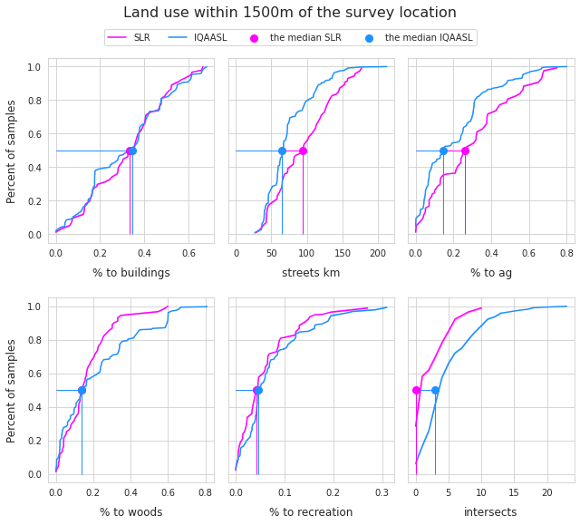
Above Distribution of number of surveys with respect to land use profile SLR - IQAASL

The sample locations in the SLR had a greater percent of land attributed to agriculture and a denser road network compared to locations in IQAASL. The percent of land attributed to woods diverges after the median at which point the locations in IQAASL had a greater percentage of land attributed to woods compared to SLR.

The population (not shown) is taken from statpop 2018 [Con]. The smallest population was 442 and the largest was 415,357. At least 50% of the samples came from municipalities with a population of 13,000 or less.

If percent of land use attributed to agriculture is a sign of urbanization, then the survey areas in 2021 were slightly more urban than 2018.

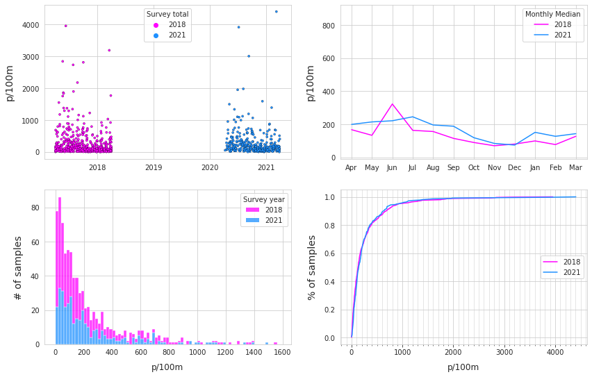
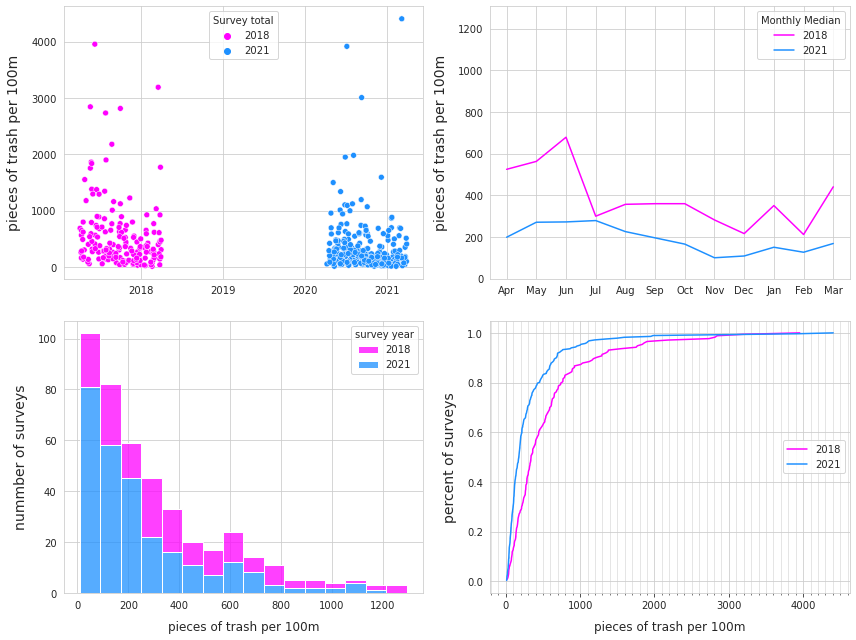
21.2. Results lakes and rivers¶

Considering only lakes and rivers that have samples in both years, there were more samples and trash collected from fewer locations in 2018 than 2021. However, on a pieces per meter basis the median was greater in 2021.

21.2.1. Distribution of results 2018 and 2021¶

Top Left: survey totals by date. Top right: median monthly survey total. bottom Left: number of samples with respect to the survey total. bottom right: empirical cumulative distribution of survey totals.

# group by survey and sum all the objects for each survey AKA: survey total
data=df.groupby(["survey year","water_name_slug","loc_date", "location", "date"], as_index=False)[unit_label].sum()
data["lakes"] = data.water_name_slug.isin(these_lakes)

# get the ecdf for both projects
ecdf_2017 = ECDF(data[data["survey year"] == "2018"][unit_label].values)
ecdf_2021 = ECDF(data[data["survey year"] == "2021"][unit_label].values)

# get the ecddf for the condition lakes in both years
l2017 = data[(data.water_name_slug.isin(these_lakes))&(data["survey year"] == "2018")].copy()
l2021 = data[(data.water_name_slug.isin(these_lakes))&(data["survey year"] == "2021")].copy()

ecdf_2017l = ECDF(l2017[unit_label].values)
ecdf_2021l = ECDF(l2021[unit_label].values)

# convenience func and dict to display table values
change_names = {"count":"# samples", "mean":F"average {unit_label}", "std":"standard deviation", "min":F"min {unit_label}",  "25%":"25%",  "50%":"50%", "75%":"75%", "max":F"max {unit_label}", "min":"min p/100", "total objects":"total objects", "# locations":"# locations", "survey year":"survey year"}

# group by survey year and use pd.describe to get basic stats
som_1720 = data.groupby("survey year")[unit_label].describe().round(2)

# add total quantity and number of unique locations
som_1720["total objects"] = som_1720.index.map(lambda x: df[df["survey year"] == x].quantity.sum())
som_1720["# locations"] = som_1720.index.map(lambda x: df[df["survey year"] == x].location.nunique())

# make columns names more descriptive
som_1720.rename(columns=(change_names), inplace=True)
ab = som_1720.reset_index()

# melt that on survey year
c_s = ab.melt(id_vars=["survey year"])

# pivot on survey year
combined_summary = c_s.pivot(columns="survey year", index="variable", values="value").reset_index()

# format for printing
combined_summary["2018"] = combined_summary["2018"].map(lambda x: F"{int(x):,}")
combined_summary["2021"] = combined_summary["2021"].map(lambda x: F"{int(x):,}")

# change the index to date
data.set_index("date", inplace=True)

# get the median monthly value
monthly_2017 = data.loc[data["survey year"] == "2018"]["p/100m"].resample("M").median()

# change the date to the name of the month for charting
months_2017 = pd.DataFrame({"month":[dt.datetime.strftime(x, "%b") for x in monthly_2017.index], unit_label:monthly_2017.values})

# repeat for 2021
monthly_2021 = data.loc[data["survey year"] == "2021"]["p/100m"].resample("M").median()
months_2021 = pd.DataFrame({"month":[dt.datetime.strftime(x, "%b") for x in monthly_2021.index], unit_label:monthly_2021.values})

# set the date intervals for the chart
months = mdates.MonthLocator(interval=1)
months_fmt = mdates.DateFormatter("%b")
years = mdates.YearLocator()

# set a y limit axis:
the_90th = np.percentile(data["p/100m"], 95)

# chart that
fig, ax = plt.subplots(2,2, figsize=(14,9), sharey=False)

# set axs and lables
axone=ax[0,0]
axtwo = ax[0,1]
axthree = ax[1,0]
axfour = ax[1,1]

axone.set_ylabel(unit_label, **ck.xlab_k14)
axone.xaxis.set_minor_locator(months)
axone.xaxis.set_major_locator(years)
axone.set_xlabel(" ")

axtwo.set_xlabel(" ")
axtwo.set_ylabel(unit_label, **ck.xlab_k14)
axtwo.set_ylim(-10, the_90th)

axthree.set_ylabel("# of samples", **ck.xlab_k14)
axthree.set_xlabel(unit_label, **ck.xlab_k)

axfour.set_ylabel("% of samples", **ck.xlab_k14)
axfour.set_xlabel(unit_label, **ck.xlab_k)

# histogram data:
data_long = pd.melt(data[["survey year", "loc_date", unit_label]],id_vars=["survey year","loc_date"], value_vars=(unit_label,), value_name="survey total")
data_long["year_bin"] = np.where(data_long["survey year"] == "2018", 0, 1)

# scatter plot of surveys both years
sns.scatterplot(data=data, x="date", y="p/100m", color="red", s=10, ec="black", hue="survey year", palette=this_palette, ax=axone)
# sns.scatterplot(data=data[data.water_name_slug.isin(these_lakes)], x="date", y="p/100m", color="red", s=34, ec="white",label="survey total", hue="survey year", palette= this_palettel, ax=axone)
axone.legend(loc="upper center", title="Survey total")

# monthly median
sns.lineplot(data=months_2017, x="month", y=unit_label, color=this_palette["2018"], label="2018", ax=axtwo)
sns.lineplot(data=months_2021, x="month", y=unit_label, color=this_palette["2021"], label="2021", ax=axtwo)
axtwo.legend(title="Monthly Median")
# histogram
sns.histplot(data=data_long, x="survey total", hue="survey year", stat="count", multiple="stack",palette=this_palette, ax=axthree, bins=[x*20 for x in np.arange(80)])

# empirical cumulative distribution
sns.lineplot(x=ecdf_2017.x, y=ecdf_2017.y, ax=axfour, color=this_palette["2018"], label="2018")
sns.lineplot(x=ecdf_2021.x, y=ecdf_2021.y, ax=axfour, color=this_palette["2021"], label="2021")
axthreel = axthree.get_legend()
axthreel.set_title("Survey year")


axfour.xaxis.set_major_locator(ticker.MultipleLocator(1000)) 
axfour.xaxis.set_minor_locator(ticker.MultipleLocator(100)) 

axfour.legend(loc="center right")
axfour.tick_params(which="both", bottom=True)
axfour.grid(visible=True, which="minor",linewidth=0.5)

plt.show()

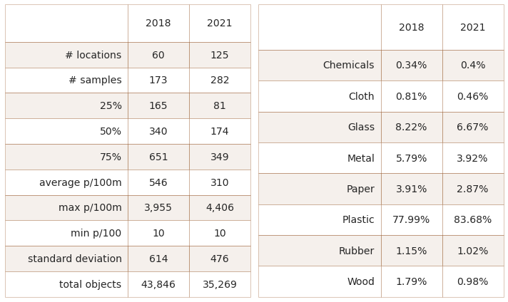
21.2.2. Summary data and material types 2018 and 2021¶

Left: summary of survey totals. Right: material type

# material totals
mat_total = df.groupby(["survey year", "code"], as_index=False).quantity.sum()

# add material type:
mat_total["mat"] = mat_total.code.map(lambda x:code_material_map.loc[x])

# the cumulative sum of material by category
mat_total = mat_total.groupby(["survey year", "mat"], as_index=False).quantity.sum()

# get the % of total and fail rate for each object from each year
# add the yearly total column
mat_total.loc[mat_total["survey year"] == "2018", "yt"] = mat_total[mat_total["survey year"] == "2018"].quantity.sum()
mat_total.loc[mat_total["survey year"] == "2021", "yt"] = mat_total[mat_total["survey year"] == "2021"].quantity.sum()

# get % of total
mat_total["pt"] =((mat_total.quantity/mat_total.yt)*100).round(2)

# format for printing:
mat_total["pt"] = mat_total.pt.map(lambda x: F"{x}%")
mat_total["quantity"] = mat_total.quantity.map(lambda x: F"{x:,}")

# pivot and rename columns
m_t = mat_total[["survey year","mat", "quantity", "pt"]].pivot(columns="survey year", index="mat", values="pt").reset_index()
m_t.rename(columns={"mat":"material", "pt":"% of total"}, inplace=True)

# put that in a table
fig, axs = plt.subplots(1, 2, figsize=(10,6))

axone = axs[0]
axtwo= axs[1]

# convenience func
sut.hide_spines_ticks_grids(axone)
sut.hide_spines_ticks_grids(axtwo)

# summary data table
a_table = sut.make_a_table(axone, combined_summary.values,  colLabels=combined_summary.columns, colWidths=[.5,.25,.25], loc="lower center", bbox=[0,0,1,1])
a_table.get_celld()[(0,0)].get_text().set_text(" ")
# material totals
second_table = sut.make_a_table(axtwo, m_t.values,  colLabels=m_t.columns, colWidths=[.5,.25,.25], loc="lower center", bbox=[0,0,1,1])

second_table.get_celld()[(0,0)].get_text().set_text(" ")

plt.tight_layout()

plt.show()

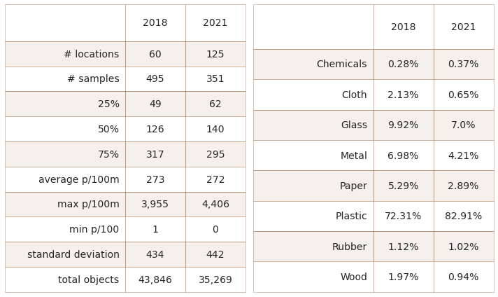
Chemicals refers to parafin wax and wood refers to treated or wood shaped for use

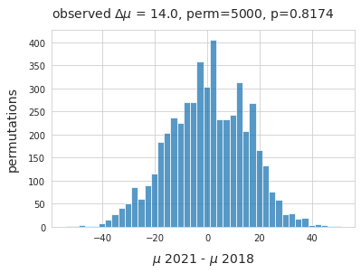
21.2.2.1. Difference of medians 2018 - 2021¶

The observed difference of the medians between the two projects is 14p/100m, differences of this magnitude would not be perceived and may be due to chance. A permutation test was conducted to test the hypothesis:

Null hypothesis: The median survey result from 2018 is not statistically different than the median from 2021. The observed difference is due to chance.

Alternate hypothesis: The median survey result from 2018 is not statistically different than the median from 2021. The observed difference in the samples is not due to chance.

Below: The distribution of the difference of medians between the two sampling periods. The survey results were shuffled and sampled 5,000 times on the survey year column. The null hypothesis can not be rejected, supporting the argument that the median survey results were approximately equal year over year.

# data for testing
data=df.copy()

# get the survey total for each survey keep the survey year column
pre_shuffle = data.groupby(["loc_date", "survey year"], as_index=False)[unit_label].sum()

# get the median from each year
observed_median = pre_shuffle.groupby("survey year")[unit_label].median()

# get the dif mu_2021 - mu_2017
observed_dif = observed_median.loc["2021"] - observed_median.loc["2018"]

# a place to store the sample statistics
new_medians=[]

# resampling:
for element in np.arange(5000):
    
    # shuffle the entire survey year column
    pre_shuffle["new_class"] = pre_shuffle["survey year"].sample(frac=1, replace=True).values
    # get the median for both "survey years"
    b=pre_shuffle.groupby("new_class").median()
    # get the change and store it    
    new_medians.append((b.loc["2018"] - b.loc["2021"]).values[0])

# calculate the empirical p
emp_p = np.count_nonzero(new_medians <= observed_dif )/ 5000

# chart the results
fig, ax = plt.subplots()

sns.histplot(new_medians, ax=ax)
ax.set_title(F"observed $\u0394\mu$ = {np.round(observed_dif, 2)}, perm=5000, p={emp_p} ", **ck.title_k14)
ax.set_ylabel("permutations", **ck.xlab_k14)
ax.set_xlabel("$\mu$ 2021 - $\mu$ 2018", **ck.xlab_k14)
plt.show()

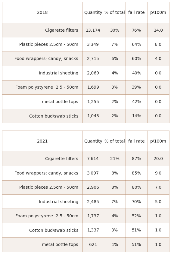
21.2.3. The most common objects year over year¶

Below: The most common objects are the ten most abundant by quantity AND/OR objects identified in at least 50% of all surveys. This accounts for 60% - 80% of all objects identified in any given survey period. The most common objects are not the same year over year. To assess the changes only the objects that were the most common in both years are included. Left: most common objects 2018, right: most common objects 2021

# code totals by project
c_totals = df.groupby(["survey year", "code"], as_index=False).agg({"quantity":"sum", "fail":"sum", unit_label:"median"})

# calculate the fail rate % of total for each code and survey year
for a_year in ["2018", "2021"]:
    c_totals.loc[c_totals["survey year"] == a_year, "fail rate"] = ((c_totals.fail/df[df["survey year"] == a_year].loc_date.nunique())*100).astype("int")
    c_totals.loc[c_totals["survey year"] == a_year, "% of total"] = ((c_totals.quantity/df[df["survey year"] == a_year].quantity.sum())*100).astype("int")
    
# get all the instances where the fail rate is > fail_rate
c_50 = c_totals.loc[c_totals["fail rate"] >= fail_rate]

# the top ten from each project
ten_2017 = c_totals[c_totals["survey year"] == "2018"].sort_values(by="quantity", ascending=False)[:10].code.unique()
ten_2021 = c_totals[c_totals["survey year"] == "2021"].sort_values(by="quantity", ascending=False)[:10].code.unique()

# combine the most common from each year with the top ten from each year
# most common 2017
mcom_2017 = list(set(c_50[c_50["survey year"]=="2018"].code.unique())|set(ten_2017))

# most common 2021
mcom_2021 = list(set(c_50[c_50["survey year"]=="2021"].code.unique())|set(ten_2021))

# the set of objects that were the most common in both years:
mcom = list(set(mcom_2017)&set(mcom_2021))

# get the data
com_2017 = c_totals[(c_totals["survey year"] == "2018")&(c_totals.code.isin(mcom))]
com_2021 = c_totals[(c_totals["survey year"] == "2021")&(c_totals.code.isin(mcom))]

# format values for table
table_data = []
chart_labels = ["2018", "2021"]
for i, som_data in enumerate([com_2017, com_2021]):
    som_data = som_data.set_index("code")
    som_data.sort_values(by="quantity", ascending=False, inplace=True)
    som_data["item"] = som_data.index.map(lambda x: code_description_map.loc[x])
    som_data["% of total"] = som_data["% of total"].map(lambda x: F"{int(x)}%")
    som_data["quantity"] = som_data.quantity.map(lambda x: F"{int(x):,}")
    som_data["fail rate"] = som_data["fail rate"].map(lambda x: F"{int(x)}%")
    som_data[unit_label] = som_data[unit_label].map(lambda x: F"{round(x,2)}")    
    table_data.append({chart_labels[i]:som_data})

# the columns needed
cols_to_use = {"item":"Item","quantity":"Quantity", "% of total":"% of total", "fail rate":"fail rate", unit_label:unit_label}

fig, axs = plt.subplots(2,1, figsize=(8,20*.6))

for i,this_table in enumerate(table_data):
    this_ax = axs[i]    
    sut.hide_spines_ticks_grids(this_ax)
    
    a_table = sut.make_a_table(this_ax, table_data[i][chart_labels[i]][cols_to_use.keys()].values,  colLabels=list(cols_to_use.values()), colWidths=[.48, *[.13]*4], bbox=[0, 0, 1, 1])
    this_ax.set_xlabel(" ")
    a_table.get_celld()[(0,0)].get_text().set_text(chart_labels[i])

    
plt.tight_layout()
plt.subplots_adjust(wspace=0.15)
plt.show()

plt.close()

21.3. Results lakes 2018 and 2021¶

The following lakes were sampled in both project years:

Zurichsee
Bielersee
Neuenburgersee
Walensee
Lac Léman
Thunersee

When considering the six lakes (above), in 2021 there were more samples and locations and greater quantities of litter collected, but the median and average were both lower with respect to 2018.

Top Left: survey totals by date, Top right: median monthly survey total, bottom Left: number of samples with respect to the survey total, bottom right: empirical cumulative distribution of survey totals

# a df with just the lakes of interest
lks_df = df[df.water_name_slug.isin(these_lakes)].copy()

# a month column
lks_df["month"] = lks_df.date.dt.month

# survey totals
lks_dt = lks_df.groupby(["survey year", "water_name_slug","loc_date","date", "month"], as_index=False)[unit_label].sum()

# locations in both years
com_locs_df = lks_df[lks_df.location.isin(both_years)].copy()

# nsamps from locations in both years
nsamps_com_locs = com_locs_df[com_locs_df["survey year"] == "2021"].groupby(["location"], as_index=True).loc_date.nunique()

# common locations surveyed in 2021
com_locs_20 = com_locs_df[com_locs_df["survey year"] == "2021"].location.unique()

# locations surveyed in 2021
locs_lakes = lks_df[lks_df["survey year"] == "2021"].location.unique()

data=lks_df.groupby(["survey year","loc_date", "date"], as_index=False)[unit_label].sum()
data.set_index("date", inplace=True)

# the empirical distributions for each year
ecdf_2017 = ECDF(data[data["survey year"] == "2018"][unit_label].values)
ecdf_2021 = ECDF(data[data["survey year"] == "2021"][unit_label].values)

# get the x,y vals for each year
ecdf_2017_x, ecdf_2017_y = ecdf_2017.x, ecdf_2017.y
ecdf_2021_x, ecdf_2021_y = ecdf_2021.x, ecdf_2021.y

the_90th = np.percentile(data[unit_label], 95)

# the monthly plots
just_2017 = data[data["survey year"] == "2018"][unit_label].resample("M").median()
monthly_2017 = pd.DataFrame(just_2017)
monthly_2017.reset_index(inplace=True)
monthly_2017["month"] = monthly_2017.date.map(lambda x: dt.datetime.strftime(x, "%b"))

just_2021 = data[data["survey year"] == "2021"][unit_label].resample("M").median()
monthly_2021 = pd.DataFrame(just_2021)
monthly_2021.reset_index(inplace=True)
monthly_2021["month"] = monthly_2021.date.map(lambda x: dt.datetime.strftime(x, "%b"))

# long form data for histogram
data_long = pd.melt(data[["survey year", "p/100m"]],id_vars=["survey year"], value_vars=("p/100m",), value_name="survey total")
data_long["year_bin"] = np.where(data_long["survey year"] == "2018", 0, 1)
data_long = data_long[data_long["survey total"] < the_90th].copy()

fig, ax = plt.subplots(2,2, figsize=(12,9), sharey=False)

# set axs and labels
axone=ax[0,0]
axtwo = ax[0,1]
axthree = ax[1,0]
axfour = ax[1,1]

axone.set_ylabel("pieces of trash per 100m", **ck.xlab_k14)
axone.set_xlabel(" ")

axone.xaxis.set_minor_locator(months)
axone.xaxis.set_major_locator(years)

axtwo.set_xlabel(" ")
axtwo.set_ylabel("pieces of trash per 100m", **ck.xlab_k14)


axthree.set_ylabel("nummber of surveys", **ck.xlab_k14)
axthree.set_xlabel("pieces of trash per 100m", **ck.xlab_k)
axtwo.set_ylim(0, the_90th)

axfour.set_ylabel("percent of surveys", **ck.xlab_k14)
axfour.set_xlabel("pieces of trash per 100m", **ck.xlab_k)

# all samples scatter
sns.scatterplot(data=data, x="date", y=unit_label, color="red", s=34, ec="white", hue="survey year", palette= this_palette, ax=axone)
axone.legend(loc="upper center", title="Survey total")

# monthly medians
sns.lineplot(data=monthly_2017, x="month", y=unit_label, color=this_palette["2018"], label=F"2018", ax=axtwo)
sns.lineplot(data=monthly_2021, x="month", y=unit_label, color=this_palette["2021"],label=F"2021",  ax=axtwo)
axtwo.legend(title="Monthly Median")

# histogram of survey results
sns.histplot(data=data_long, x="survey total", hue="survey year", stat="count", multiple="stack", palette=this_palette, ax=axthree)

# ecdfs
sns.lineplot(x=ecdf_2017_x, y=ecdf_2017_y, ax=axfour, color=this_palette["2018"], label="2018")
sns.lineplot(x=ecdf_2021_x, y=ecdf_2021_y, ax=axfour, color=this_palette["2021"], label="2021")

axfour.xaxis.set_major_locator(ticker.MultipleLocator(1000)) 
axfour.xaxis.set_minor_locator(ticker.MultipleLocator(100)) 
axfour.legend(loc="center right")
axfour.tick_params(which="both", bottom=True)
axfour.grid(visible=True, which="minor",linewidth=0.5)



plt.tight_layout()
plt.show()

Left: summary of survey totals, right: material type

# group by survey year and use pd.describe to get basic stats
som_1720 = lks_dt.groupby("survey year")[unit_label].describe().round(2)

# add total quantity and number of unique locations
som_1720["total objects"] = som_1720.index.map(lambda x: df[df["survey year"] == x].quantity.sum())
som_1720["# locations"] = som_1720.index.map(lambda x: df[df["survey year"] == x].location.nunique())

# make columns names more descriptive
som_1720.rename(columns=(change_names), inplace=True)
ab = som_1720.reset_index()

# melt that on survey year
c_s = ab.melt(id_vars=["survey year"])

# pivot on survey year
combined_summary = c_s.pivot(columns="survey year", index="variable", values="value").reset_index()

# format for printing
combined_summary["2018"] = combined_summary["2018"].map(lambda x: F"{int(x):,}")
combined_summary["2021"] = combined_summary["2021"].map(lambda x: F"{int(x):,}")

# material totals
mat_total = lks_df.groupby(["survey year", "code"], as_index=False).quantity.sum()

# add material type:
mat_total["mat"] = mat_total.code.map(lambda x:code_material_map.loc[x])

# the most common codes for each year
mat_total = mat_total.groupby(["survey year", "mat"], as_index=False).quantity.sum()

# get the % of total and fail rate for each object from each year
# add the yearly total column
mat_total.loc[mat_total["survey year"] == "2018", "yt"] = mat_total[mat_total["survey year"] == "2018"].quantity.sum()
mat_total.loc[mat_total["survey year"] == "2021", "yt"] = mat_total[mat_total["survey year"] == "2021"].quantity.sum()

# get % of total
mat_total["pt"] =((mat_total.quantity/mat_total.yt)*100).round(2)

# format for printing:
mat_total["pt"] = mat_total.pt.map(lambda x: F"{x}%")
mat_total["quantity"] = mat_total.quantity.map(lambda x: F"{x:,}")

m_t = mat_total[["survey year","mat", "quantity", "pt"]].pivot(columns="survey year", index="mat", values="pt").reset_index()
m_t.rename(columns={"mat":"material", "pt":"% of total"}, inplace=True)

# put that in a table
fig, axs = plt.subplots(1, 2, figsize=(10,6))

axone = axs[0]
axtwo= axs[1]

sut.hide_spines_ticks_grids(axone)
sut.hide_spines_ticks_grids(axtwo)

# summary data table
a_table = sut.make_a_table(axone, combined_summary.values,  colLabels=combined_summary.columns, colWidths=[.5,.25,.25], loc="lower center", bbox=[0,0,1,1])
a_table.get_celld()[(0,0)].get_text().set_text(" ")
# material totals
second_table = sut.make_a_table(axtwo, m_t.values,  colLabels=m_t.columns, colWidths=[.5,.25,.25], loc="lower center", bbox=[0,0,1,1])

second_table.get_celld()[(0,0)].get_text().set_text(" ")

plt.tight_layout()

plt.show()

plt.tight_layout()

plt.show()

<Figure size 432x288 with 0 Axes>

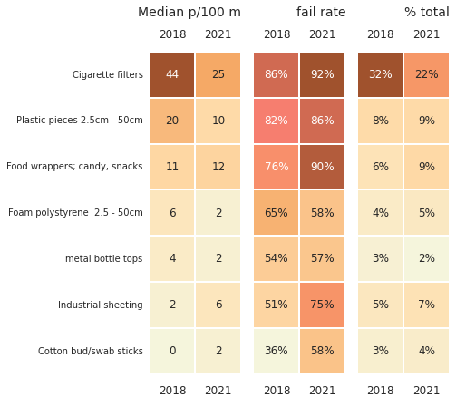
21.3.1. Lakes: results most common objects from 2018¶

Below: the most common objects were 71% of all objects counted in 2018 versus 60% in 2021. Cigarette filters and fragmented plastic pieces were recorded at almost double the rate in 2018 versus 2021.

Lakes: key indicators of the most common objects 2018 - 2021

# compare the key indicators of the most common objects
lks_codes = lks_df[lks_df.code.isin(mcom)].copy()
lks_codes = lks_df[lks_df.code.isin(mcom)].groupby(["code", "survey year"], as_index=False).agg({unit_label:"median", "quantity":"sum", "fail":"sum", "loc_date":"nunique"})

# get fail rate and % of total
for a_year in ["2021", "2018"]:
    lks_codes.loc[lks_codes["survey year"] == a_year, "fail rate"] = lks_codes.fail/lks_df[lks_df["survey year"]==a_year].loc_date.nunique()
    lks_codes.loc[lks_codes["survey year"] == a_year, "% of total"] = lks_codes.quantity/lks_df[lks_df["survey year"]==a_year].quantity.sum()

lks_codes["d"] = lks_codes.code.map(lambda x: code_description_map.loc[x])


a = lks_codes.pivot(columns="survey year", values=unit_label, index="d")
b = lks_codes.pivot(columns="survey year", values="fail rate", index="d").astype(float)
c = lks_codes.pivot(columns="survey year", values="% of total", index="d")

# plot that
fig = plt.figure(figsize=(8, 12))

# use gridspec to position
spec = GridSpec(ncols=8, nrows=2, figure=fig)
axone = fig.add_subplot(spec[:,1:3])
axtwo = fig.add_subplot(spec[:,3:5])
axthree = fig.add_subplot(spec[:,5:7])

# get an order to assign each ax
an_order = a.sort_values(by="2018", ascending=False).index

# index axtwo and and axthree to axone
axone_data = a.sort_values(by="2018", ascending=False)
axtwo_data = b.sort_values(by="2018", ascending=False).reindex(an_order)
axthree_data = c.sort_values(by="2018", ascending=False).reindex(an_order)

# pieces per meter



sns.heatmap(axone_data, cmap=cmap2, annot=True, annot_kws={"fontsize":12},  ax=axone, square=True, cbar=False, linewidth=.05,  linecolor="white")
axone.tick_params(**dict(labeltop=True, labelbottom=True, pad=12, labelsize=12), **ck.no_xticks)
axone.set_xlabel(" ")
axone.set_title("Median p/100 m",**ck.title_k14r)

# fail rate


sns.heatmap(axtwo_data, cmap=cmap2, annot=True, annot_kws={"fontsize":12}, fmt=".0%", ax=axtwo, square=True,  cbar=False, linewidth=.05,  linecolor="white")
axtwo.tick_params(**dict(labeltop=True, labelbottom=True, pad=12, labelsize=12), **ck.no_xticks)
axtwo.tick_params(labelleft=False, left=False)
axtwo.set_xlabel(" ")
axtwo.set_title("fail rate", **ck.title_k14r)

# percent of total
sns.heatmap(axthree_data, cmap=cmap2, annot=True, annot_kws={"fontsize":12}, fmt=".0%", ax=axthree, square=True,  cbar=False, linewidth=.05,  linecolor="white")
axthree.tick_params(**dict(labeltop=True, labelbottom=True, pad=12, labelsize=12), **ck.no_xticks)
axthree.tick_params(labelleft=False, left=False)
axthree.set_xlabel(" ")
axthree.set_title("% total", **ck.title_k14r)

for anax in [axone, axtwo, axthree]:
    anax.set_ylabel("")

plt.subplots_adjust(wspace=0.3)

plt.show()

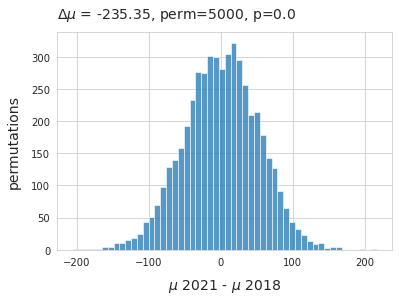
21.3.2. Difference of mean survey total¶

When considering only lakes the difference of medians is inversed, less litter was observed in 2021 than 2018 and the difference of means is much larger in favor of 2018. Suggesting that at the lake level there was a decrease in observed quantities.

Null hypothesis: The mean of the survey results for lakes from 2018 is not statistically different than the mean for 2021. The observed difference is due to chance.

Alternate hypothesis: The mean survey results for lakes in 2018 is not the same in 2021. The observed difference in the samples is significant.

Below: The distribution of the difference of means between the two sampling periods. The survey results were shuffled and sampled 5,000 times on the survey year column. The null hypothesis could be rejected, supporting the initial observation that there was less observed in 2021 than 2018.

# data for testing
data=df[df.water_name_slug.isin(these_lakes)].copy()

# get the survey total for each survey keep the survey year column
pre_shuffle = data.groupby(["survey year", "loc_date"], as_index=False)[unit_label].sum()

# get the mean for each survey year
observed_mean = pre_shuffle.groupby("survey year")[unit_label].mean()

# get the diff
observed_dif = observed_mean.loc["2021"] - observed_mean.loc["2018"]

new_means=[]
# resampling:
for element in np.arange(5000):
    
    # shuffle the survey year column
    pre_shuffle["new_class"] = pre_shuffle["survey year"].sample(frac=1).values
    # get the means for both years
    b=pre_shuffle.groupby("new_class").mean()
    # get the change and store it
    new_means.append((b.loc["2021"] - b.loc["2018"]).values[0])

# calculate p
emp_p = np.count_nonzero(new_means <= observed_dif )/ 5000

# chart the results
fig, ax = plt.subplots()

sns.histplot(new_means, ax=ax)
ax.set_title(F"$\u0394\mu$ = {np.round(observed_dif, 2)}, perm=5000, p={emp_p} ", **ck.title_k14)
ax.set_ylabel("permutations", **ck.xlab_k14)
ax.set_xlabel("$\mu$ 2021 - $\mu$ 2018", **ck.xlab_k14)
plt.show()

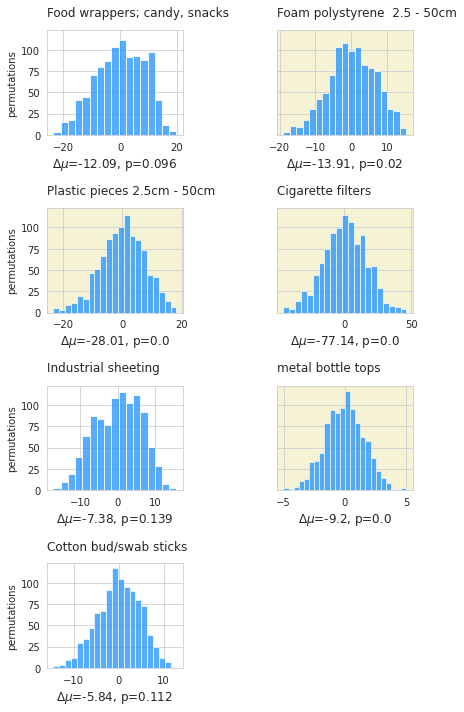
21.3.2.1. Difference of means most common objects¶

The observed difference of means between the two sampling periods was -235p/100m. The most common objects are approximately equal to 60% of the total. Changes in the daily total may be reflected in the daily totals of the most common objects as well.

Test one:

Null hypothesis: The mean of the of the survey results of the most common objects from 2018 is the same as 2021. The observed difference is due to chance.

Alternate hypothesis: The mean of the survey results of the most common objects from 2018 is different than 2021. The observed difference in the samples is significant.

if p < 0.05 = yellow: the difference is statistically significant.

Below: The observed difference in means between the two years could be in part explained by the decrease in the quantities of cigarettes, foam polystyrene, metal bottle tops and fragmented plastics.

# data testing
data=df[df.water_name_slug.isin(these_lakes)].copy()

# data to resample
pre_shuffle = data[data.code.isin(mcom)].groupby(["survey year", "loc_date", "code"], as_index=False)[unit_label].sum()

# the observed mean from each year
observed_mean = pre_shuffle.groupby(["survey year", "code"])[unit_label].mean()

# get the differences from one year to the next: check the inverse
observed_dif = observed_mean.loc["2021"] - observed_mean.loc["2018"]
inv_diff = observed_mean.loc["2018"] - observed_mean.loc["2021"]

# number of shuffles
perms = 1000

new_means=[]
# resample
for a_code in mcom:
    
    # store the test statisitc
    cdif = []
    
    # code data
    c_data = pre_shuffle[pre_shuffle.code == a_code].copy()
    for element in np.arange(perms):
        # shuffle labels
        c_data["new_class"] = c_data["survey year"].sample(frac=1).values
        b=c_data.groupby("new_class").mean()
        cdif.append((b.loc["2021"] - b.loc["2018"]).values[0])
    
    # calculate p
    emp_p = np.count_nonzero(cdif <= (observed_dif.loc[a_code])) / perms

    # store that result
    new_means.append({a_code:{"p":emp_p,"difs":cdif}})    

# chart the results
fig, axs = plt.subplots(4,2, figsize=(6,10), sharey=True)

for i,code in enumerate(mcom):
    
    # set up the ax
    row = int(np.floor((i/2)%4))
    col =i%2
    ax=axs[row, col]
    
    # data for charts
    data = new_means[i][code]["difs"]
    
    # pvalues
    p=new_means[i][code]["p"]
   
    
    # set the facecolor based on the p value
    
    if p < 0.05:
        ax.patch.set_facecolor("palegoldenrod")
        ax.patch.set_alpha(0.5)        
    # plot that    
    sns.histplot(data, ax=ax, color=this_palette["2021"])
    
    ax.set_title(code_description_map.loc[code], **ck.title_k)
    ax.set_xlabel(F"$\u0394\mu$={np.round(observed_dif.loc[code], 2)}, p={new_means[i][code]['p']}", fontsize=12)
    ax.set_ylabel("permutations")

# hide the unused axs
sut.hide_spines_ticks_grids(axs[3,1])

# get some space for xaxis label
plt.tight_layout()
plt.subplots_adjust(hspace=0.7, wspace=.7)
plt.show()

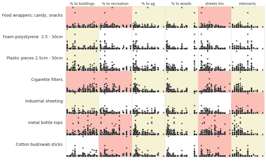
21.3.3. Land use profile: Spearmans ranked correlation¶

The land use features were previously calculated to compare the survey locations. To test the statistical significance of land use on beach litter survey results the survey totals and locations from both projects were considered as one group. The survey results of the most common objects were tested against the measured land use features.

Spearmans \(\rho\) or Spearmans ranked correlation coefficient is a non-parametric test of rank correlation between two variables [Wikd] [Inn]. The test results are evaluated at p<0.05 and 454 samples, SciPy is used to implement the test [scc].

Red/rose is a positive association: p<0.05 AND \(\rho\) > 0
yellow is a negative association: p<0.05 AND \(\rho\) < 0
white medians that p>0.05, there is no statistical basis to assume an association

Below: An association suggests that survey totals for that object will change in relation to the amount of space attributed to that feature, or in the case of roads or river intersections, the quantity. The magnitude of the relationship is not defined, and any association is not linear.

corr_data = lks_df[(lks_df.code.isin(mcom))].copy()

# keys to the column names
some_keys = {
    "% to buildings":"lu_build",
    "% to agg":"lu_agg",
    "% to woods":"lu_woods",
    "% to recreation":"lu_rec",
    "% to trans":"lu_trans",
    "% to meadow":"lu_m",
    "str_rank":"lu_trans"
}

fig, axs = plt.subplots(len(mcom),len(luse_exp), figsize=(len(luse_exp)+7,len(mcom)+1), sharey="row")

for i,code in enumerate(mcom):
    data = corr_data[corr_data.code == code]
    for j, n in enumerate(luse_exp):
        # each grid is its own axis with a scatterplot
        ax=axs[i, j]
        ax.grid(False)
        ax.tick_params(axis="both", which="both",bottom=False,top=False,labelbottom=False, labelleft=False, left=False)
       
        if i == 0:
            ax.set_title(F"{n}")
        else:
            pass
        
        if j == 0:
            ax.set_ylabel(F"{code_description_map[code]}", rotation=0, ha="right", **ck.xlab_k14)
            ax.set_xlabel(" ")
        else:
            ax.set_xlabel(" ")
            ax.set_ylabel(" ")
        _, corr, a_p = sut.make_plot_with_spearmans(data, ax, n)
        
        # assign the facecolor based on the value of p and rho
        if a_p < 0.05:
            if corr > 0:
                ax.patch.set_facecolor("salmon")
                ax.patch.set_alpha(0.5)
            else:
                ax.patch.set_facecolor("palegoldenrod")
                ax.patch.set_alpha(0.5)

plt.tight_layout()
plt.subplots_adjust(wspace=0, hspace=0)
# plt.savefig(F"{project_directory}/test_one.jpg", dpi=300)
plt.show()

21.3.3.1. Interpret Spearmans \(\rho\)¶

Interpreting results for the most common objects

A positive association medians that the land use attribute or feature had increased survey results when compared to other locations. This may be due to a covariance of attributes, either way a positive association is a signal that the survey locations are near a zone of accumulation or a source. This signal should be assessed along with the other key indicators of survey locations that have similar land use profiles. In general locations that fit the criteria could be considered as both a source and an area of accumulation for any objects that are positively associated.

A negative association medians that the land use feature or attribute does not facilitate the accumulation of the object. This result is common for agricultural areas and woods on the national level. A negative association is a signal that the locations are not a zone of accumulation for the object.

No or few association means that the land use features had no effect on the accumulation of that object. The survey results of the most common objects with no or few associations fall into two characteristics:

Ubiquitous: high fail rate, high pieces per meter. Found at consistent rates through out the survey area indifferent of land use
Transient: low fail rate, high quantity, high pieces per meter, few associations. Found occasionally in large quantities at specific locations

21.4. Conclusion¶

21.4.1. On balance no change¶

The summary statistics and the results of the difference of medians test imply that there was no statistically measurable change on the national scale from one project to the next. The 95% CI of the median survey total in 2021 was 137 - 188p/100m ( section Calculating Baselines ). The median result for 2018 was 125p/100m with a CI of 112p/100m to 146p/100m, which includes the lower bound of the median from 2021. However, the difference of means for the most common objects suggest a more realistic and dynamic result:

There was a statistically significant decrease in four of seven most common objects from both years:
- cigarette ends
- metal bottle caps
- plastic fragments
- foam fragments

The decrease in tobacco and bottle tops is likely the result of pandemic related restrictions that marked 2021. These results suggest that perceived local decreases in litter quantities were most likely the result of a general decline in usage as opposed to a sweeping change in behavior. Consequently the survey results for list 1 items will most likely return to 2018 levels as pandemic related restrictions are relaxed and usage patterns return to normal.

The decreases in fragmented foams and plastics is likely due to a difference in protocols between the two years.

21.4.2. Protocols matter¶

There was a key difference between the two projects:

The 2021 protocol counts all visible objects and classifies fragments by size
The 2018 protocol limited the object counts to items greater than or equal to 2.5cm in length

The total amount of plastic pieces collected in 2021 is 7,400 or 18p/100m and 5,563 or 5p/100m foamed plastic fragments. There were 3,662 plastic pieces between 0.5cm and 2.5cm removed in 2021, equal to the total amount recorded in 2018. The same for foamed plastics between 0.5cm and 2.5cm, see Lakes and rivers.

The difference in protocol and the results from 2021 cast doubt on the likelihood of any decrease of fragmented plastics and foamed plastics from 2018 to 2021. Foamed plastics and fragmented plastics are objects whose original use is unknown but the material can be distinguished. Fragmented plastics and foamed plastics greater than 0.5cm are 27% of the total survey results for the lakes in 2021. Studies in the Meuse/Rhine delta show that these small, fragmented objects make up large portions of the total abundance [vE].

Allowing surveyors to use a broader range of object codes increases the accuracy of the total survey count and adds levels of differentiation between similar materials. For example, expanded polystyrene is an object that fragments easily. Whether or not surveyors are finding a few larger pieces > 20cm or thousands of pieces < 10mm is an important detail if reducing these objects in the environment is the goal.

Reduced cost and increased access are another result of a harmonized protocol. The procedures used by the SLR and IQAASL were almost identical, except for the size limit it can be assumed that the samples were collected under similar conditions. The SLR data gives the results of over 1,000 observations by approximately 150 people and the IQAASL data gives the results of 350 observations from approximately 10 people. Both methods have weaknesses and strengths that address very diverse topics:

experience of surveyor
consistency of survey results
oversight
intended use of data
allocation of resources

All of these topics should be considered with each project, as well as stewardship of the data. Regardless of the differences, we were able to build on the model proposed by the SLR and add to the shared experience.

21.4.3. Plastic lids¶

Plastic lids are separated into three categories during the counting process:

drink, food
household cleaners etc..
unknown

As group plastic lids make up 2% of the total objects in 2018 and 3% in 2021. Drink lids were ~51% of all lids found in 2018, 45% in 2021. On a pieces per meter basis there was a decrease in the amount of drink lids and an increase of non-drink lids from 2018 - 2021.

21.4.4. Land use profile¶

The land use profile for each location was calculated using the same data for both years. When survey results from both years are considered as a group the results from Spearmans 𝜌 lend support to the SLR conclusions in 2018 that survey results were elevated in urban and suburban environments and this was also true in 2021. At the same time the ubiquitous nature of fragmented plastics, industrial sheeting and expanded foams noted in The land use profile was likely prevalent in 2018.

The amount of land attributed to recreational activities are locations near the survey site designed to accommodate groups of people for various activities. The positive association of tobacco and food/drink related products with this land attribute could be interpreted as the result of temporary increases in population near the survey site.

21.4.5. Conclusions¶

The samples from both projects were taken from locations, in some cases the same location, that had similar levels of infrastructure and economic development. A common protocol was used in both projects, the samples were collected by two different groups and managed by two different associations.

From 2018 - 2021 there was a statistically significant change, a decrease in the number of objects directly related to behavior at the survey site. This indicates that any perceived decreases were in locations that had a higher % of land attributed to buildings and lower % of land attributed to agriculture or woods.

Locations with an opposing or different land use profile (less buildings, more agriculture or woods) will most likely not have experienced any decrease at all. For locations near river interchanges or major discharge points there would be no perceivable difference from 2018 - 2021 and increases in fragmented plastics, expanded foams and industrial sheeting were likely. Both the test of difference of medians of the most common objects and the results from Spearmans \(\rho\) of survey results support this conclusion.

Both survey years show peak survey results in June - July (annex) and lows in November. The possible causes for the peaks and troughs are different depending on the object in question. Food and tobacco objects are more prevalent during the summer season because of increased use. Objects like fragmented plastics depend more on hydrological conditions and the peak discharge rate of the biggest rivers in this study are from May - July( section Shared responsibility ).

Future surveys should include visible items of all sizes. Data aggregation can be done at the server using defined rules based on known relationships. The total count is a key indicator in all statistics that rely on count data, for modeling purposes it is essential.

21.5. Annex¶

Pariticipating organizations

Precious plastic leman
Association pour la sauvetage du Léman
Geneva international School
Solid waste management: École polytechnique fédéral Lausanne

21.5.1. Lakes: monthly median common objects:¶

All lakes were sampled in all months in both projects. In 2018 the minimum samples per month was 12 and the maximum was 17 compared to a minimum of 17 and max of 34 in 2021.

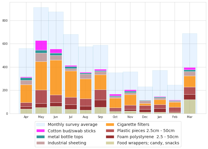
Lakes 2018: monthly average survey result most common objects

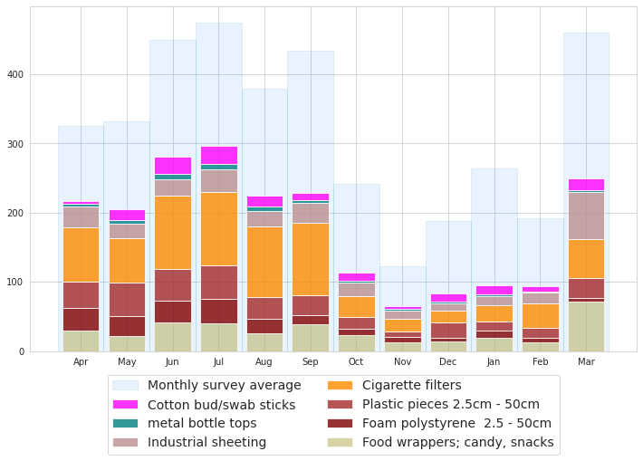
Lakes 2021: monthly average survey result most common objects

21.5.1.1. Survey locations ¶

	latitude	longitude	city
slug
aabach	47.220989	8.940365	Schmerikon
anarchy-beach	46.447216	6.859612	La Tour-de-Peilz
augustmutzenbergstrandweg	46.686640	7.689760	Spiez
baby-plage-geneva	46.208558	6.162923	Genève
baby-plage-ii-geneve	46.208940	6.164330	Genève
bain-des-dames	46.450507	6.858092	La Tour-de-Peilz
baye-de-montreux-g	46.430834	6.908778	Montreux
bielersee_vinelz_fankhausers	47.038398	7.108311	Vinelz
boiron	46.491030	6.480162	Tolochenaz
camp-des-peches	47.052812	7.074053	Le Landeron
camping-gwatt-strand	46.727140	7.629620	Thun
cully-plage	46.488887	6.741396	Bourg-en-Lavaux
delta-park	46.720078	7.635304	Spiez
erlach-camping-strand	47.047159	7.097854	Erlach
evole-plage	46.989477	6.923920	Neuchâtel
flibach-river-right-bank	47.133742	9.105461	Weesen
gals-reserve	47.046272	7.085007	Gals
gasi-strand	47.128442	9.110831	Weesen
grand-clos	46.387746	6.843686	Saint-Gingolph
hauterive-petite-plage	47.010797	6.980304	Hauterive (NE)
impromptu_cudrefin	46.964496	7.027936	Cudrefin
la-pecherie	46.463919	6.385732	Allaman
la-petite-plage	46.785054	6.656877	Yverdon-les-Bains
lacleman_gland_lecoanets	46.402811	6.281959	Gland
le-pierrier	46.439727	6.888968	Montreux
ligerz-strand	47.083979	7.135894	Ligerz
luscherz-plage	47.047955	7.151242	Lüscherz
luscherz-two	47.047519	7.152829	Lüscherz
maladaire	46.446296	6.876960	La Tour-de-Peilz
mols-rocks	47.114343	9.288174	Quarten
muhlehorn-dorf	47.118448	9.172124	Glarus Nord
mullermatte	47.133339	7.227907	Biel/Bienne
murg-bad	47.115307	9.215691	Quarten
nidau-strand	47.127196	7.232613	Nidau
nouvelle-plage	46.856646	6.848428	Estavayer
oyonne	46.456682	6.852262	La Tour-de-Peilz
parc-des-pierrettes	46.515215	6.575531	Saint-Sulpice (VD)
pecos-plage	46.803590	6.636650	Grandson
pfafikon-bad	47.206766	8.774182	Freienbach
plage-de-cheyres	46.818689	6.782256	Cheyres-Châbles
plage-de-st-sulpice	46.513265	6.570977	Saint-Sulpice (VD)
pointe-dareuse	46.946190	6.870970	Boudry
preverenges	46.512690	6.527657	Préverenges
preverenges-le-sout	46.508905	6.534526	Préverenges
quai-maria-belgia	46.460156	6.836718	Vevey
rastplatz-stampf	47.215177	8.844286	Rapperswil-Jona
rocky-plage	46.209737	6.164952	Genève
ruisseau-de-la-croix-plage	46.813920	6.774700	Cheyres-Châbles
schmerikon-bahnhof-strand	47.224780	8.944180	Schmerikon
seeflechsen	47.130223	9.103400	Glarus Nord
seemuhlestrasse-strand	47.128640	9.295100	Walenstadt
signalpain	46.786200	6.647360	Yverdon-les-Bains
strandboden-biel	47.132510	7.233142	Biel/Bienne
sundbach-strand	46.684386	7.794768	Beatenberg
thun-strandbad	46.739939	7.633520	Thun
thunersee_spiez_meierd_1	46.704437	7.657882	Spiez
tiger-duck-beach	46.518256	6.582546	Saint-Sulpice (VD)
tolochenaz	46.497509	6.482875	Tolochenaz
untertenzen	47.115260	9.254780	Quarten
versoix	46.289194	6.170569	Versoix
vidy-ruines	46.516221	6.596279	Lausanne
villa-barton	46.222350	6.152500	Genève
walensee_walenstadt_wysse	47.121828	9.299552	Walenstadt
weissenau-neuhaus	46.676583	7.817528	Unterseen
zuerichsee_richterswil_benkoem_2	47.217646	8.698713	Richterswil
zuerichsee_staefa_hennm	47.234643	8.769881	Stäfa
zuerichsee_waedenswil_colomboc_1	47.219547	8.691961	Richterswil
zurcher-strand	47.364200	8.537420	Zürich
zurichsee_kusnachterhorn_thirkell-whitej	47.317685	8.576860	Küsnacht (ZH)
zurichsee_wollishofen_langendorfm	47.345890	8.536155	Zürich
la-morges	46.504063	6.494099	Morges
lac-leman-hammerdirt	46.450389	6.858234	La Tour-de-Peilz
lacleman_gland_kubela	46.402869	6.281936	Gland
lacleman_vidy_santie	46.518318	6.589608	Lausanne
neuenburgersee_cudrefin_mattera	46.962709	7.025968	Cudrefin
zuerichsee_maennedorf_vanderkaadene	47.254754	8.687504	Männedorf
zuerichsee_zurich_kullg	47.353957	8.550474	Zürich
zurichsee-feldeggstr-banningersand	47.359392	8.547368	Zürich

More and less since 2018

Contents