2. The Alps and the Jura¶

The Alps and the Jura (les Alpes) is a survey area configured and managed by the Summit Foundation. The Summit Foundation has conducted clean up events throughout the Swiss Alps for many years. Included in the 2021 events were a series of litter-surveys conducted in parallel to the regularly scheduled events. Summit foundation had two questions with respect to IQAASL:

How can data collection be integrated into the current business model?
How do surveys conducted on mountain trails compare to those on the waters edge?

The purpose of clean-up events is to remove as much litter as possible from a defined area, the limits on how much can be removed is related to the resources at hand. A litter survey is used to identify and maintain a count of the objects within a defined area. In this sense a clean-up event is approaching the litter problem from the perspective of attenuation or mitigation and litter-surveys provide the data necessary to improve prevention.

2.1. Survey methods¶

In total there were twenty litter-surveys conducted by Summit foundation. Initially two methods were selected:

Survey a section of trail for a defined distance and width
Survey the installations at the arrival/departure of the lift line

The survey procedure remains the same under both conditions:

A section of trail or surface area is measured
All visible pollutants are removed counted and classified.
The results and dimensions are recorded

The difference between the two methods is the way the limits of survey area are defined. When a trail is used the limits of the survey area are defined by the trail itself, not the surveyor. In the summertime the barriers and signs that mark out the areas for lift lines have all been removed, making it difficult for the surveyor to accurately determine the correct limits.

2.2. Survey area cumulative totals¶

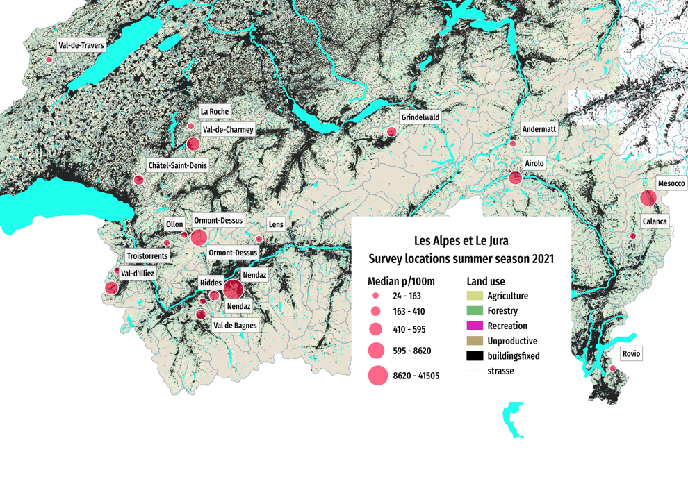
Below: The Alpes and Jura survey area summer 2021. Marker diameter = the mean survey result in pieces of litter per 100 meters (p/100m).

# define the final survey data set here:
# combined the alps and the lakes and rivers data
predata = pd.concat([aldata, sdata])

# remove the prefix from the location names
predata["location"] = predata["location"].map(lambda x: sut.get_rid_of_ix(x, prefix="clean-up-tour-"))

# assign loc_date and make date stamp
predata["loc_date"] = list(zip(predata.location, predata["date"]))
predata["date"] = pd.to_datetime(predata["date"])

# remove prefixes from the alps location names
fd = predata[predata.river_bassin == "les-alpes"].copy()
sd = predata[predata.river_bassin != "les-alpes"]

# merge it back in with the rest
a_data = pd.concat([fd, sd])

# scale the streets to kilometers
a_data["streets"] = a_data.streets.astype("int")

# the totals for each survey and the locations in the feature data
fd_dt=fd.groupby(["loc_date", "date","month", "location"], as_index=False).agg(agg_pcs_quantity)

# survey totals
dt_all = a_data.groupby(["loc_date","location","river_bassin", "date"], as_index=False).agg(agg_pcs_quantity)

# the unique locations and samples
t = {"samples":fd.loc_date.nunique(),
     "locations":fd.location.unique(),
     "nlocations":fd.location.nunique(),
     "fdtotalq": fd.quantity.sum()
    }

# gather the municpalities and the population:
fd_pop_map = dfBeaches.loc[fd.location.unique()][["city","population"]].copy()
fd_pop_map.drop_duplicates(inplace=True)
fd_pop_map.set_index("city", drop=True, inplace=True)

t.update({"nmunis":len(fd_pop_map.index)})

# fancy print to jupyter:
obj_string = "{:,}".format(t["fdtotalq"])
surv_string = "{:,}".format(t["samples"])
pop_string = "{:,}".format(int(fd_pop_map.sum()[0]))

date_quantity_context = F"Between {start_date[:-3]} and {end_date[:-3]}, a total of {obj_string } objects  were removed and identified over the course of {surv_string} surveys."
geo_context = F"This includes {t['nlocations']} different locations in {t['nmunis']} different municipalities with a combined population of {pop_string}."
munis_joined = ", ".join(sorted(fd_pop_map.index))

# put that all together:
lake_string = F"""
{date_quantity_context} {geo_context }

\n\n >{munis_joined}"""

Between 2020-03 and 2021-09, a total of 7,776 objects were removed and identified over the course of 20 surveys. This includes 20 different locations in 18 different municipalities with a combined population of 70,606.

Airolo, Andermatt, Calanca, Châtel-Saint-Denis, Grindelwald, La Roche, Lens, Mesocco, Nendaz, Ollon, Ormont-Dessus, Riddes, Rovio, Troistorrents, Val de Bagnes, Val-d'Illiez, Val-de-Charmey, Val-de-Travers

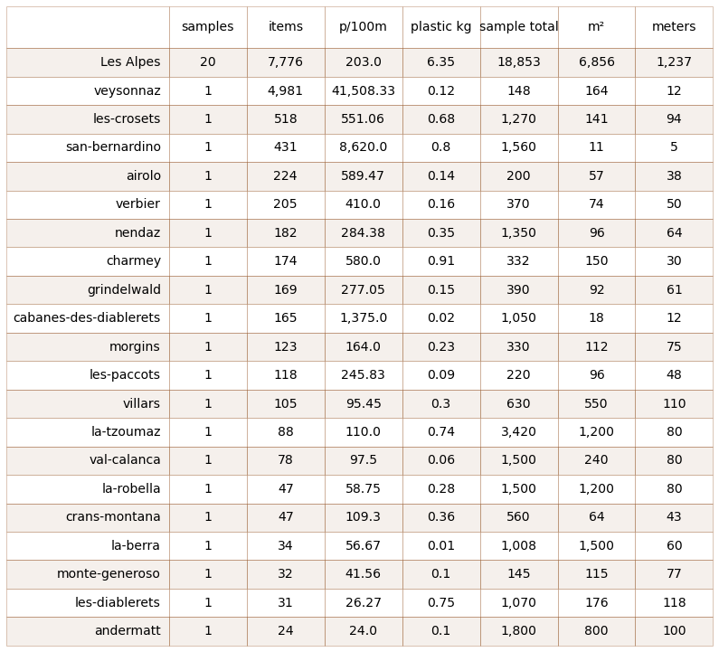
2.2.1. Litter sample totals¶

Below: The aggregated results from the litter surveys. This does not include the event totals, see next section.

# gather the dimensional data for the time frame from dfDims
# match records to survey data
# the dimensional data, remove prefix and reassemble
fd_dims = dfDims[(dfDims.river_bassin == "les-alpes")&(dfDims.date >= start_date)&(dfDims.date <= end_date)].copy()
fd_dims["location"] = fd_dims.location.apply(lambda x: x.replace("clean-up-tour-", ""))
fd_dims["loc_date"] = list(zip(fd_dims.location, fd_dims.date))

# map the daily totals to the survey dimensions
q_map = fd_dt[["loc_date", "quantity"]].set_index("loc_date").quantity
fd_dims["quantity"] = fd_dims.loc_date.map(lambda x: q_map.loc[[x]].values[0])

# get the pieces per meter
fd_dims[unit_label] = ((fd_dims.quantity/fd_dims["length"])*reporting_unit).round(2)

# make a loc_date column 
fd_dims["loc_date"] = list(zip(fd_dims.location, fd_dims.date))

agg_for_table = {
    "quantity":"sum",
    unit_label:"mean",
    "total_w":"sum",
    "mac_plast_w":"sum",
    "mic_plas_w":"sum",
    "area":"sum",
    "length":"sum",
    "num_parts_other":"sum",
    "num_parts_staff":"sum",
    "time_minutes":"sum"
    
}

# the table of cumulative values
dims_table = fd_dims.groupby(["location"]).agg(agg_for_table )

# collect the number of samples from the survey total data:
for name in dims_table.index:
    dims_table.loc[name, "samples"] = fd_dt[fd_dt.location == name].loc_date.nunique()

# get the sum of all the samples
dims_table.loc[level_names[0]]= dims_table.sum(numeric_only=True, axis=0)

# take the median pcs_m of all the samples
dims_table.loc[level_names[0], unit_label] = fd_dt.groupby(["location"])[unit_label].sum().median()

# for display
dims_table.sort_values(by=["quantity"], ascending=False, inplace=True)

new_col_names={
    "quantity":"items",
    "total_w":"total kg", 
    unit_label:unit_label, 
    "mac_plast_w":"plastic kg", 
    "mic_plas_w":"sample total", 
    "area":"m²", 
    "length":"meters"
}


dims_table.rename(columns=new_col_names, inplace=True)

# order the columns
dims_table = dims_table[["samples", *dims_table.columns[:-1]]]

# format kilos
dims_table["plastic kg"] = dims_table["plastic kg"]/1000

# format for printing
dims_table.rename(columns={"num_parts_other":"participants", "num_parts_staff":"staff", "time_minutes":"time"}, inplace=True)

# numerical types and columns
tints = ["samples", "items", "total kg", "sample total", "m²", "participants", "staff", "time", "meters"]
twodec = [unit_label, "plastic kg" ]

# apply formatting
dims_table[tints] = dims_table[tints].astype("int")
dims_table[twodec] = dims_table[twodec].round(2)
dims_table["time"] = (dims_table["time"]/60).astype("int")

# apply string formatting:
commas = ["items","total kg", "sample total", "meters", "m²", unit_label]
dims_table[commas] = dims_table[commas].applymap(lambda x: F"{x:,}")

# table one
# data = dims_table.reset_index()
table_one = dims_table[["samples", "items",unit_label,"plastic kg","sample total", "m²", "meters"]].copy()
table_one.reset_index(inplace=True)

# make table
fig, ax = plt.subplots(figsize=(14, 13))
sut.hide_spines_ticks_grids(ax)
a_table = sut.make_a_table(ax,table_one.values , colLabels=table_one.columns, colWidths=[.23, *[.11]*7], bbox=[0, 0, 1, 1], bottom_row=True)
a_table.get_celld()[(0,0)].get_text().set_text(" ")
a_table.set_fontsize(14)
plt.show()

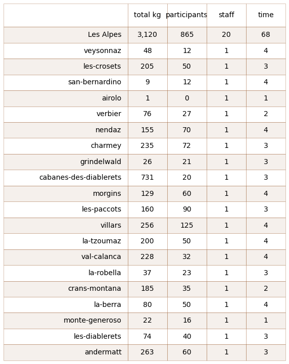
2.2.2. Event totals¶

Below: The total amount of trash collected in kilograms, the number of participants and staff and the time to complete the survey.

# table two event totals
table_two = dims_table[["total kg", "participants","staff", "time"]].copy()
table_two.reset_index(inplace=True, )

# make a table
fig, axs = plt.subplots(figsize=(10,13))
sut.hide_spines_ticks_grids(axs)

a_table = sut.make_a_table(axs, table_two.values, colLabels=table_two.columns, colWidths=[.44, *[.14]*4])
a_table.get_celld()[(0,0)].get_text().set_text(" ")
a_table.set_fontsize(14)

plt.show()
plt.tight_layout()
plt.close()

2.3. Land use profile of the survey locations¶

The land use profile is the percent of total area attributed to each land use category within a 1500m radius of each survey location.

% to buildings
% to agriculture
% to forestry
% to recreation

Streets are reported as the total number of kilometers of streets within the 1500m radius. Intersects are an ordinal ranking of the number of rivers/canals that intersect a lake within 1500m of the survey location.

The ratio of the number of samples completed at the different land use profiles is an objective indicator of the overall environmental and economic conditions that the samples were taken in. The distribution of the land use profile of all the surveys from the IQAASL project is used as a reference value.

See the section The land use profile for more details.

# explanatory variables:
luse_exp = ["% to buildings", "% to recreation", "% to agg", "% to woods", "streets", "intersects"]

# columns needed
use_these_cols = ["loc_date" ,"% to buildings", "% to trans", "% to recreation", "% to agg", "% to woods","population","location","streets", "intersects", "groupname","code"]

# the land use data from all other locations
datax = sd.groupby(use_these_cols[:-2], as_index=False).agg(agg_pcs_quantity)

# work off the copy
data = fd.groupby(use_these_cols[:-2], as_index=False).agg(agg_pcs_quantity)

sns.set_style("whitegrid")


fig, axs = plt.subplots(2, 3, figsize=(9,8), sharey="row")

for i, n in enumerate(luse_exp):
    r = i%2
    c = i%3
    ax=axs[r,c]   
    # get the empirical distribution of the independent variable
    all_surveys = ECDF(datax[n].values)
    les_alpes = ECDF(data[n].values)
        
    # plot that
    sns.lineplot(x=all_surveys.x, y=all_surveys.y, ax=ax, color=a_color, label=level_names[1])
    # plot that
    sns.lineplot(x=les_alpes.x, y=les_alpes.y, ax=ax, color="magenta", label=level_names[0])
    the_median = data[n].median()
    
    # get its position reference the surrounding survey area
    a = (stats.percentileofscore(les_alpes.x, the_median))/100
    
    # plot the median and drop horzontal and vertical lines
    ax.scatter([the_median], a, color="red",s=50, linewidth=2, zorder=100, label=level_names[0])
    ax.vlines(x=the_median, ymin=0, ymax=a, color="red", linewidth=2)
    ax.hlines(xmax=the_median, xmin=0, y=a, color="red", linewidth=2)
    
    # save the handels and labels but remove them from the ax    
    handles, labels = ax.get_legend_handles_labels()
    ax.get_legend().remove()
    
    # format the % of total on the xaxis:
    if i <= 3:
        if c == 0:            
            ax.set_ylabel("Ration of samples", **ck.xlab_k)
        ax.xaxis.set_major_formatter(ticker.PercentFormatter(1.0, 0, "%"))        
    else:
        pass
    ax.set_xlabel(n, **ck.xlab_k)

plt.tight_layout()
plt.subplots_adjust(top=.9, hspace=.3)
plt.suptitle("Land use within 1500m of the survey location", ha="center", y=1, fontsize=16)
fig.legend(handles, labels, bbox_to_anchor=(.5,.94), loc="center", ncol=3)        
plt.show()

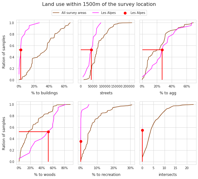
Above: The locations in the Alps survey area had a higher percentage of land attributed to forestry and aggriculture and a lower percentage of land attributed to buildings and recreation than the locations in IQAASL.

The aggregated results demonstrate the difference between the two survey methods. The three locations with the highest p/100m also have the shortest length. In the case of Cabanes-des-Diablerets the meter² is equal to the length, suggesting that a small area was surveyed around a structure or building. Veysonnaz is located at the end of a ski lift line.

The difference in methods produces markedly different results. Furthermore, these two locations were selected specifically for inventory because of the surveyor’s previous experiences. Due to the differences in dimensions and methods the survey results from Veysonnaz, San-Beranardino and Cabanes-des-Diablerets are not considered in the proceeding analysis.

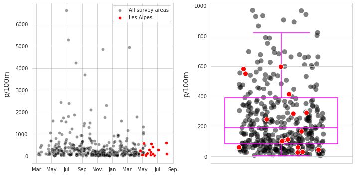
2.4. Distribution of survey results¶

Left: All samples lakes/rivers and walking trails, 2020-03 through 2021-09, n=403. Right: Distribution of survey results, outliers removed.

remove = ["veysonnaz", "cabanes-des-diablerets", "san-bernardino"]

# the feature data without the three locations
wt_data = fd[~fd.location.isin(remove)].copy()

# the daily totals of like samples
wt_dt =fd_dt[~fd_dt.location.isin(remove)].copy()

# all the data without the three locations
a_data = a_data[~a_data.location.isin(remove)]

# the 17 like sample locations
nvsn = wt_dt.location.unique()

# make a df of survey totals with date as index
# the daily survey totals of all the data for the survey period
a_dt = a_data.groupby(["loc_date", "date","location"], as_index=False).agg(agg_pcs_quantity)

# only the surveys from all other survey areas
dts_date = a_dt[(~a_dt.location.isin([*nvsn, *remove]))].copy()
# months locator, can be confusing
# https://matplotlib.org/stable/api/dates_api.html
months_fmt = mdates.DateFormatter("%b")

fig, axs = plt.subplots(1,2, figsize=(10,5))

ax = axs[0]

# there is a big value in here, that should be seen.
sns.scatterplot(data=dts_date, x="date", y=unit_label, color="black", alpha=0.4, label=level_names[1], ax=ax)
sns.scatterplot(data=wt_dt, x="date", y=unit_label, color="red", s=34, ec="white",label=level_names[0], ax=ax)

ax.set_xlabel("")
ax.set_ylabel(unit_label, **ck.xlab_k14)

# ax.tick_params(axis="x", which="both", bottom=False )
ax.xaxis.set_major_formatter(months_fmt)

axtwo = axs[1]

box_props = {
    "boxprops":{"facecolor":"none", "edgecolor":"magenta"},
    "medianprops":{"color":"magenta"},
    "whiskerprops":{"color":"magenta"},
    "capprops":{"color":"magenta"}
}
sns.boxplot(data=dts_date, y=unit_label, color="black",  ax=axtwo, showfliers=False, **box_props, zorder=1)
sns.stripplot(data=dts_date[dts_date[unit_label] <= 1000], s=10, y=unit_label, color="black", ax=axtwo, alpha=0.5, jitter=0.3, zorder=0)
sns.stripplot(data=wt_dt, y=unit_label, color="red", s=10, ec="white",linewidth=1, ax=axtwo, jitter=0.3, zorder=2)

axtwo.set_xlabel("")
axtwo.set_ylabel(unit_label, **ck.xlab_k14)

axtwo.tick_params(which="both", axis="x", bottom=False)

plt.tight_layout()
plt.show()
plt.close()

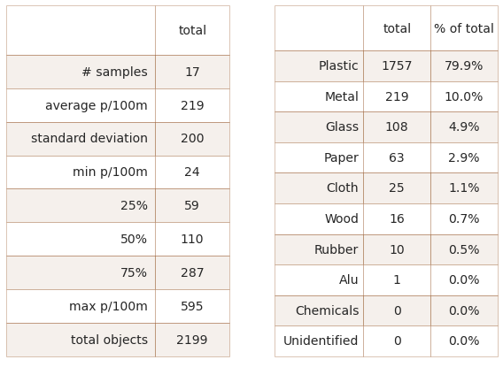
2.4.1. Summary data and material types¶

Left: Walking trails summary of survey totals. Right: Walking trails material type and percent of total.

# get the basic statistics from pd.describe
cs = wt_dt[unit_label].describe().round(2)

# add project totals
cs["total objects"] = fd[~fd.location.isin(remove)].quantity.sum()

# change the names
csx = sut.change_series_index_labels(cs, sut.create_summary_table_index(unit_label, lang="EN"))

# format the text
combined_summary = sut.fmt_combined_summary(csx, nf=[])

# the material totals
code_totals = sut.the_aggregated_object_values(wt_data, agg=agg_pcs_median, description_map=code_description_map, material_map=code_material_map)    
code_totals.sort_values(by="quantity", ascending=False)

fd_mat_totals = sut.the_ratio_object_to_total(code_totals)

fd_mat_totals = sut.fmt_pct_of_total(fd_mat_totals)
fd_mat_totals = sut.make_string_format(fd_mat_totals)

fd_mat_t = fd_mat_totals[["material", "quantity", "% of total"]].values

# make tables
fig, axs = plt.subplots(1,2, figsize=(8,6))

# summary table
# names for the table columns
a_col = [level_names[0], "total"]

axone = axs[0]
sut.hide_spines_ticks_grids(axone)

table_two = sut.make_a_table(axone, combined_summary,  colLabels=a_col, colWidths=[.5,.25,.25],  bbox=[0,0,1,1], **{"loc":"lower center"})
table_two.get_celld()[(0,0)].get_text().set_text(" ")
table_two.set_fontsize(14)

# material table
axtwo = axs[1]
axtwo.set_xlabel(" ")
sut.hide_spines_ticks_grids(axtwo)

# column names for display
cols_to_use = {"material":"material","quantity":"total", "% of total":"% of total"}

table_three = sut.make_a_table(axtwo, fd_mat_t,  colLabels=list(cols_to_use.values()), colWidths=[.4, .3,.3],  bbox=[0,0,1,1], **{"loc":"lower center"})
table_three.get_celld()[(0,0)].get_text().set_text(" ")
table_three.set_fontsize(14)

plt.tight_layout()
plt.subplots_adjust(wspace=0.2)
plt.show()

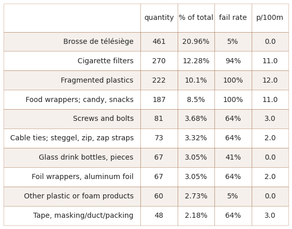
2.4.2. The most common objects¶

The most common objects are the ten most abundant by quantity found AND/OR any object that was identified in at least 50% of all the surveys.

# code totals for les Alps not including veysonnaz
code_totals.rename(columns={"groupname":"utility"}, inplace=True)

# objects with a fail rate of > 50% in the survey area
most_common = code_totals[code_totals["fail rate"] >= 50].sort_values(by="quantity", ascending=False)

# the top ten by quantity
most_abundant = code_totals.sort_values(by="quantity", ascending=False)[:10]

# merge with most_common and drop duplicates
m_common = pd.concat([most_abundant, most_common]).drop_duplicates()

# get percent of total
m_common_percent_of_total = m_common.quantity.sum()/code_totals.quantity.sum()

# format values for table
m_common["item"] = m_common.index.map(lambda x: code_description_map.loc[x])
m_common["% of total"] = m_common["% of total"].map(lambda x: F"{x}%")
m_common["quantity"] = m_common.quantity.map(lambda x: "{:,}".format(x))
m_common["fail rate"] = m_common["fail rate"].map(lambda x: F"{x}%")
m_common[unit_label] = m_common[unit_label].map(lambda x: F"{np.ceil(x)}")

# final table wt_data
cols_to_use = {"item":"item","quantity":"quantity", "% of total":"% of total", "fail rate":"fail rate", unit_label:unit_label}
walking_trails = m_common[cols_to_use.keys()].values

# figure caption
rb_string = F"""
*__Below:__ Walking trails most common objects: fail rate >/= {a_fail_rate}%  and/or top ten by quantity. 
Combined, the ten most abundant objects represent {int(m_common_percent_of_total*100)}% of all objects found, {unit_label}: median survey value.*
"""
md(rb_string)

Below: Walking trails most common objects: fail rate >/= 50% and/or top ten by quantity. Combined, the ten most abundant objects represent 69% of all objects found, p/100m: median survey value.

fig, axs = plt.subplots(figsize=(10,len(m_common)*.8))

sut.hide_spines_ticks_grids(axs)

table_three = sut.make_a_table(axs, walking_trails,  colLabels=list(cols_to_use.values()), colWidths=[.48, .13,.13,.13, .13],  bbox=[0,0,1,1], **{"loc":"lower center"})
table_three.get_celld()[(0,0)].get_text().set_text(" ")
table_three.set_fontsize(14)

plt.show()
plt.tight_layout()
plt.close()

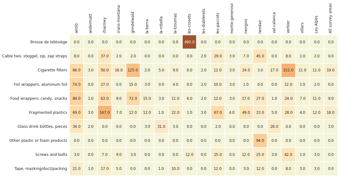
2.4.3. Most common objects results by survey location¶

Below: Walking trails most common objects: median p/100m.

# aggregated survey totals for the most common codes for all the water features 
m_common_st = wt_data[wt_data.code.isin(m_common.index)].groupby(["location", "loc_date","code"], as_index=False).agg(agg_pcs_quantity)
m_common_ft = m_common_st.groupby(["location", "code"], as_index=False)[unit_label].median()

# map the desctiption to the code
m_common_ft["item"] = m_common_ft.code.map(lambda x: code_description_map.loc[x])

# pivot that
m_c_p = m_common_ft[["item", unit_label, "location"]].pivot(columns="location", index="item")

# quash the hierarchal column index
m_c_p.columns = m_c_p.columns.get_level_values(1)

# the aggregated totals for the survey area
m_c_p[level_names[0]]= sut.aggregate_to_code(wt_data[wt_data.code.isin(m_common.index)], code_description_map,name=level_names[0])

# a_s_a = a_data[(a_data["date"] >= start_date)&(a_data["date"] <= end_date)&(a_data.code.isin(m_common.index))].groupby(["water_name_slug", "loc_date", "code"], as_index=False).agg(agg_pcs_quantity)
m_c_p[level_names[1]] = sut.aggregate_to_code(a_data[a_data.code.isin(m_common.index)], code_description_map,name=level_names[1])

# chart that
fig, ax  = plt.subplots(figsize=(len(m_c_p.columns)*.8,len(m_c_p)*.9))

axone = ax
sns.heatmap(m_c_p, ax=axone,  annot=True,vmax=300, annot_kws={"fontsize":12}, cmap=cmap2, fmt=".1f", square=True, cbar=False, linewidth=.1, linecolor="white")

axone.set_xlabel("")
axone.set_ylabel("")
axone.tick_params(labelsize=12, which="both", axis="both", labeltop=True, labelbottom=False)

plt.setp(axone.get_xticklabels(), rotation=90)

plt.tight_layout()
plt.show()
plt.close()

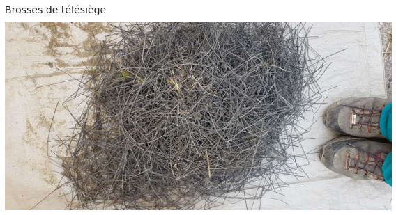
Below: Brosse de télésiège/ski-lift brushes, used to remove ice and snow from ski lifts can get separated from the installation, producing thousands of heavy gage plastic filaments.

teamv = PILImage.open("resources/images/alpes_valaisanne/veysonnaz_brosse.jpg")

# display images
fig, ax = plt.subplots(figsize=(8,4.5))

axone=ax
sut.hide_spines_ticks_grids(axone)
axone.imshow(teamv);
axone.set_title("Brosses de télésiège", **ck.title_k14)

plt.tight_layout()
plt.show()

2.5. Utility of the objects found¶

The utility type is based on the utilization of the object prior to it being discarded or item description if the original use is undetermined. Identified objects are classified into one of the predefined categories. The categories are grouped according to utilization or item description.

wastewater: items released from water treatment plants includes items likely toilet flushed
micro plastics (< 5mm): fragmented plastics and pre-production plastic resins
infrastructure: items related to construction and maintenance of buildings, roads and water/power supplies
food and drink: all materials related to consuming food and drink
agriculture: primarily industrial sheeting i.e., mulch and row covers, greenhouses, soil fumigation, bale wraps. Includes hard plastics for agricultural fencing, flowerpots etc.
tobacco: primarily cigarette filters, includes all smoking related material
recreation: objects related to sports and leisure i.e., fishing, hunting, hiking etc.
packaging non food and drink: packaging material not identified as food, drink nor tobacco related
plastic fragments: plastic pieces of undetermined origin or use
personal items: accessories, hygiene and clothing related

See the annex for the complete list of objects identified, includes descriptions and group classification. The section Code groups describes each code group in detail and provides a comprehensive list of all objects in a group.

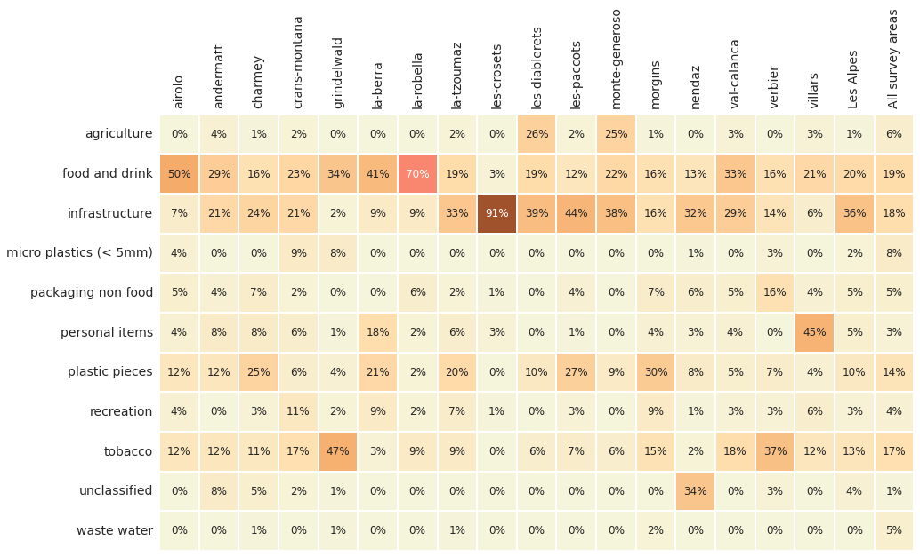
Below: Walking trails utility of objects found: % of total by water feature. Fragmented objects with no clear identification remain classified by size.

# the median survey total and % of total for codegroups
cg_t = wt_data.groupby(["loc_date", "location","groupname"], as_index=False).agg(agg_pcs_quantity)

# aggregate all that for each water feature
cg_t = cg_t.groupby(["location", "groupname"], as_index=False).agg({unit_label:"median", "quantity":"sum"})

# quantity per water feature
cg_tq = cg_t.groupby("location").quantity.sum()

# assign the water feature total to each record
for a_feature in cg_tq.index:
    cg_t.loc[cg_t.location == a_feature, "f_total"] = cg_tq.loc[a_feature]

# get the percent of total for each group for each water feature
cg_t["pt"] = (cg_t.quantity/cg_t.f_total).round(2)

# pivot that
data_table = cg_t.pivot(columns="location", index="groupname", values="pt")

# make a column for the survey area and all data
data_table[level_names[0]]= sut.aggregate_to_group_name(wt_data,name=level_names[0])
data_table[level_names[1]]= sut.aggregate_to_group_name(sd, name=level_names[1])

# chart that
fig, ax = plt.subplots(figsize=(len(data_table.columns)*.8,len(data_table)*.9))

axone = ax
sns.heatmap(data_table , ax=axone, cmap=cmap2, annot=True, annot_kws={"fontsize":12}, cbar=False, fmt=".0%", linewidth=.1, square=True, linecolor="white")

axone.set_xlabel("")
axone.set_ylabel("")
axone.tick_params(labelsize=14, which="both", axis="both", labeltop=True, labelbottom=False)

plt.setp(axone.get_xticklabels(), rotation=90, fontsize=14)
plt.setp(axone.get_yticklabels(), rotation=0, fontsize=14)

plt.show()

# median p/50m solve cg_t for unit_label
data_table = cg_t.pivot(columns="location", index="groupname", values=unit_label)

# survey area median
data_table[level_names[0]] = sut.aggregate_to_group_name(fd, name=level_names[0], val="med")

# all survey area median
data_table[level_names[1]] = sut.aggregate_to_group_name(sd, unit_label=unit_label, name=level_names[1], val="med" )

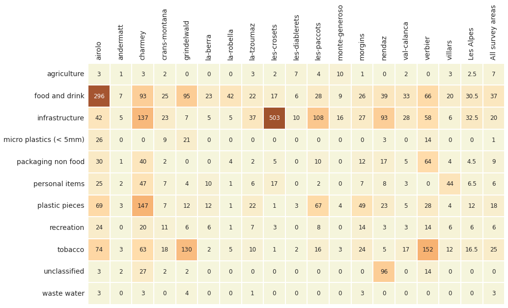
Below: Walking trails utility of objects found: median p/100m.

2.5.1. Percentile ranking of survey results with respect to land use¶

# get the percentile ranking under each condition:
# define land use ranges based on the sample data
l_f = ["% to agg", "% to woods", "population"]

this_range = (fd[l_f[0]].min(), fd[l_f[0]].max())
this_range_w = (fd[l_f[1]].min(), fd[l_f[1]].max())
this_range_p = (fd[l_f[2]].min(), fd[l_f[2]].max())

# apply them to all the data
# one test for agg -- a dominant land use feature of the sample data
some_data = a_data[(a_data[l_f[0]] >= this_range[0])&(a_data[l_f[0]] <= this_range[1])].copy()

# one test for woods -- the dominant land use feature of the sample data
some_data_w = a_data[(a_data[l_f[1]] >= this_range_w[0])&(a_data[l_f[1]] <= this_range_w[1])].copy()

# one test for population -- 
some_data_p = a_data[(a_data[l_f[2]] >= this_range_p[0])&(a_data[l_f[2]] <= this_range_p[1])].copy()

# remove Alps valaisannes
some_data = some_data[~some_data.location.isin(fd.location.unique())].copy()
some_data_w = some_data_w[~some_data_w.location.isin(fd.location.unique())].copy()
some_data_p = some_data_p[~some_data_p.location.isin(fd.location.unique())].copy()

# the number of samples and locations that have similar land use profiles as AV:
# agg to loc_date for each criteria
# data for charting and comparing
data=some_data.groupby(["loc_date","location",l_f[0]], as_index=False)[unit_label].sum()
data_w =some_data_w.groupby(["loc_date","location",l_f[1]], as_index=False)[unit_label].sum()
data_p = some_data_p.groupby(["loc_date","location",*l_f[1:]], as_index=False)[unit_label].sum()

# get the percentile ranking for each location under each condtion:
table_data = {}
for i,x in enumerate(nvsn):
    this_num = wt_dt.loc[wt_dt.location == x, unit_label].values[0]
    a = (stats.percentileofscore(data[unit_label].to_numpy(), this_num))
    b = (stats.percentileofscore(data_p[unit_label].to_numpy(), this_num))
    c = (stats.percentileofscore(data_w[unit_label].to_numpy(), this_num))
    table_data.update({x:{"agriculture":a, "woods":b, "population":c}})

# make df and format
t_data = pd.DataFrame(table_data)
t_data = t_data.astype("int")
t_data.reset_index(inplace=True)
t_data.rename(columns={"index":"variable"}, inplace=True)
t_data.set_index("variable", inplace=True, drop=True)

fig, ax = plt.subplots(figsize=(len(nvsn)*.8,5))

axone = ax
sns.heatmap(t_data , ax=axone, cmap=cmap2, vmax=300, annot=True, annot_kws={"fontsize":12}, fmt="g", cbar=False, linewidth=.1, square=True, linecolor="white")

axone.set_ylabel("")
axone.tick_params(labelsize=14, which="both", axis="both", labeltop=True, labelbottom=False)

plt.setp(axone.get_xticklabels(), rotation=90, fontsize=14)
plt.setp(axone.get_yticklabels(), rotation=0, fontsize=14)

plt.show()

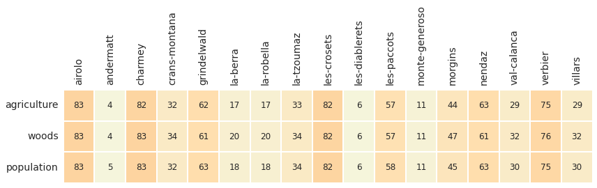
Above: The ranking of the alpes survey locations with respect to land use. For example, the survey results at Airolo were greater than 83% of all the surveys (lakes, rivers and alpes). At Andermatt the survey results are lower than 95% of all surveys with a comparable land use profile.

2.6. Discussion¶

2.6.1. Alps survey results compared to shoreline surveys¶

The median value is 110 p/100m for the 17 locations that met the length and width criteria in the Alps survey area, less than the median value of all the other survey areas (189p/100m). Objects related to consumption such as food, drink and tobacco were a smaller percent of the total and had a lower p/100m rate compared to locations along water systems. This difference could be in part due to the low levels of urbanization that characterizes the Alps survey area with respect to all other survey areas.

Objects related to infrastructure are 36% of the total or twice the rate encountered when all the survey areas are considered. This is largely attributed to ski-lift brush filaments identified in substantial quantities at Les-Crosets. Ski lift brushes are used to remove the snow from the top of covered ski-lift-chairs as they approach the embarkation site. Similar to industrial pellets or expanded foam beads in the aquatic environment, ski brush pieces will likely be a recurring item to be identified in occasionally large quantities at very specific sites.

The ratio of infrastructure objects to food and tobacco objects is almost 1, results like these are typical of environments that have a more developed infrastructure, see Shared Responsibility. Fragmented plastics are found at rates similar to the other survey areas. Cable ties and masking tape are new additions to the most common list, both objects are found on the shoreline but at rates below 50%.

Recall that these surveys were conducted along the ski-lift line or a walking trail on the domain of a ski-area. While use may be greater in winter, many domains are excellent vtt and hiking areas, establishing a use case year-round for these regions.

2.6.1.1. Most common objects¶

The most common objects are 74% of the total identified. Cigarette ends did not exceed the national median in the Alpes survey area, however there were significant values recorded at Verbier, Grindelwald and Airolo. Specific items from the infrastructure group are represented such as:

screws and bolts
cable ties
masking tape
bricks and pipes

However, the absence of expanded or extruded polystyrene from the Alps survey areas most common list is a sharp contrast to all other survey areas where this product alone is approximately 13% of the total, see Lakes and rivers.

2.6.2. Implementing litter surveys in the existing business model¶

A clean-up event covers a relatively large geographic area compared to a beach-litter survey. Volunteers to these events are drawn by the opportunity to take care of the environment AND enjoy some moderate exercise in the company of others. Beach-litter surveys do not offer the same type of activity level and may not be of interest to all volunteers.

Implementing beach litter surveys means offering the experience to volunteers at the event but maintaining the resources internally to ensure that the survey is completed according to protocol. This includes identifying, counting and entering data. Summit foundation was able to do this by ensuring that there was one person present at each event that could complete the survey.

The surveyors from summit foundation preferred to sample along the lift lines and starting at the arrival and departure of ski lifts. Samples taken this way follow the flow of the event: downhill and within the areas of high traffic.

Samples that were taken around buildings or other installations produced higher survey results. Confirming what Summit foundation members had identified in previous years. From these experiences the Project manager, Téo Gursoy, explained:

Indeed, the surveyors concentrate mainly on the sections under the chairlifts, gondolas or at the departure and arrival of these installations which are highly frequented places.

In some instances, the density of the objects is so great that the surveyor felt compelled to concentrate on one area by expanding the width of the survey area. M Gursoy described what happened when a surveyor happened on a location that had large quantities of ski-lift brushes:

However, the surveyor started the trail section at the arrival station of the gondola. The ski-lift brushes quickly caught the surveyor”s attention who decided to focus on this area alone in order to find out how many of them could be found in this type of area…

The survey results around infrastructure or buildings are not indicative of the state of the environment throughout the domain. Surveys around these structures tend to have higher counts, however they make up only a small portion of the total land use.

Adjustments had to be made to the software and reporting scheme in order to handle the different types of data that are produced from clean-up events. That included creating new identification codes for specific objects that are found in the Alps survey area. Furthermore, Summit foundation provided the resources so that one foundation staff member could be trained using the project protocol and software.

2.6.3. Conclusions¶

The surveys conducted along the trails and lift lines in the Alps survey area produced data that was very similar to the data produced from surveys done on the shoreline. However, when surveyors focused their attention around specific infrastructure items the survey counts return extreme values. Survey results on the shoreline would produce the same results if surveys were only conducted at locations where high litter counts were more probable.

Food and drink objects are only 11% of the total objects found compared to 36% from the other survey areas. However, infrastructure objects are 75% of the total in the Alps versus 18% at all other survey areas. This is in part due to the difference in human presence when compared to locations at lower altitudes where human presence is a constant throughout the year, thus more of a pressure from food and tobacco objects as opposed to infrastructure.

This first project also demonstrated the feasibility of combining monitoring with popular events. In preparation to monitoring, the members of both teams exchanged ideas and sorted samples together. This permitted both organizations to better understand each other and determine baseline services that could be provided while collecting data for a national report:

Assist in the collection and identification
Assist in the data entry
Provide charts, graphs and data that can be used by the participating organizations

A beach-litter survey requires 2-4 hours to complete, depending on how many different objects there are. This resource was not accounted for in the operating budget of either organization. Therefore, Summit foundation provided the coordination and infrastructure and hammerdirt provided an additional surveyor and IT support.

The data provided allows for direct comparisons between locations, provided that the same survey method is used. The abundance of infrastructure items relative to food and tobacco items is indicative of surveys completed in rural locations. How well this data compares to surveys done on the shoreline needs to be explored further. However, cigarette ends, broken glass, fragmented plastics and snack wrappers are among the most common items found on the shoreline.

We thank all the members of Summit Foundation for their help and specifically Olivier Kressmann and Téo Gursoy.

2.7. Annex¶

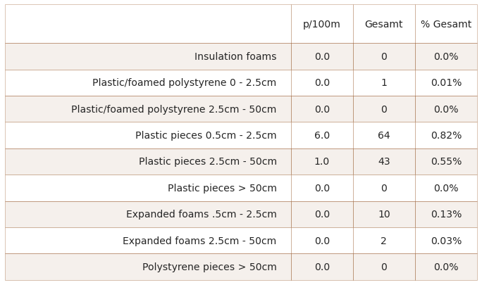
2.7.1. Fragmented foams and plastics by size group¶

The table below contains the components of Gfoam and Gfrags. Objects labeled “Expanded foams” are grouped as Gfoam the rest are grouped as Gfrags for analysis.

Below: fragmented foams and plastics by size group. Median {unit_label}, number of pieces, percent of total.

## collect the data before aggregating foams for all locations in the survye area
h=pd.read_csv("resources/checked_alpes_survey_data_be.csv")

# remove prefix
h["location"] = h["location"].map(lambda x: sut.get_rid_of_ix(x, prefix="clean-up-tour-"))

# remove prefixes from survey data
lAlps = h[h.river_bassin == bassin_name][["loc_date","code","location","river_bassin","groupname", "quantity", "pcs_m"]].copy()

# convert to reporting unit
lAlps[unit_label]= (lAlps.pcs_m*100).round(2)

# the fragmented plastics and foams
some_foams = ["G81", "G82", "G83", "G74"]
some_frag_plas = list(lAlps[lAlps.groupname == "plastic pieces"].code.unique())

# get just the foams and plastics and aggregate to code
conditions = ((lAlps.code.isin([*some_frag_plas, *some_foams]))&(~lAlps.location.isin(remove)))
fd_frags_foams = lAlps[conditions].groupby(["loc_date","code"], as_index=False).agg(agg_pcs_quantity)
fd_frags_foams = fd_frags_foams.groupby("code", as_index=False).agg(agg_pcs_median)

# add code description and format for printing
fd_frags_foams["item"] = fd_frags_foams.code.map(lambda x: code_description_map.loc[x])
fd_frags_foams["% of total"] = (fd_frags_foams.quantity/fd.quantity.sum()*100).round(2)
fd_frags_foams["% of total"] = fd_frags_foams["% of total"].map(lambda x: F"{x}%")
fd_frags_foams["quantity"] = fd_frags_foams["quantity"].map(lambda x: F"{x:,}")

# table data
data = fd_frags_foams[["item",unit_label, "quantity", "% of total"]].copy()
data.rename(columns={"quantity":"Gesamt", "% of total":"% Gesamt"}, inplace=True)

fig, axs = plt.subplots(figsize=(12,len(data)*.8))
sut.hide_spines_ticks_grids(axs)

this_table = sut.make_a_table(axs, data.values,  colLabels=data.columns, colWidths=[.6, .13, .13, .13], bbox=[0, 0, 1, 1])
this_table.get_celld()[(0,0)].get_text().set_text(" ")
this_table.set_fontsize(14)

plt.show()
plt.tight_layout()
plt.close()

2.7.2. Land use profile of survey locations¶

# get the land use profile of AV
lu_prof = fd[["location","% to buildings", "% to recreation", "% to agg", "% to woods","population","streets"]].drop_duplicates()

# format for printing
lu_prof.loc[:,lu_prof.columns[1:-2]] = lu_prof.loc[:,lu_prof.columns[1:-2]].applymap(lambda x: F"{int((x*100))}%")
lu_prof.loc[:, lu_prof.columns[5:]] = lu_prof.loc[:, lu_prof.columns[5:]].applymap(lambda x: F"{int(x):,}")

# put that to a table
data=lu_prof.copy()

fig, axs = plt.subplots(figsize=(13,len(table_one)*.6))
sut.hide_spines_ticks_grids(axs)

this_table = sut.make_a_table(axs, data.values,  colLabels=data.columns, colWidths=[.22, *[.13]*6], bbox=[0, 0, 1, 1])
this_table.get_celld()[(0,0)].get_text().set_text(" ")
this_table.set_fontsize(14)

plt.tight_layout()
plt.show()

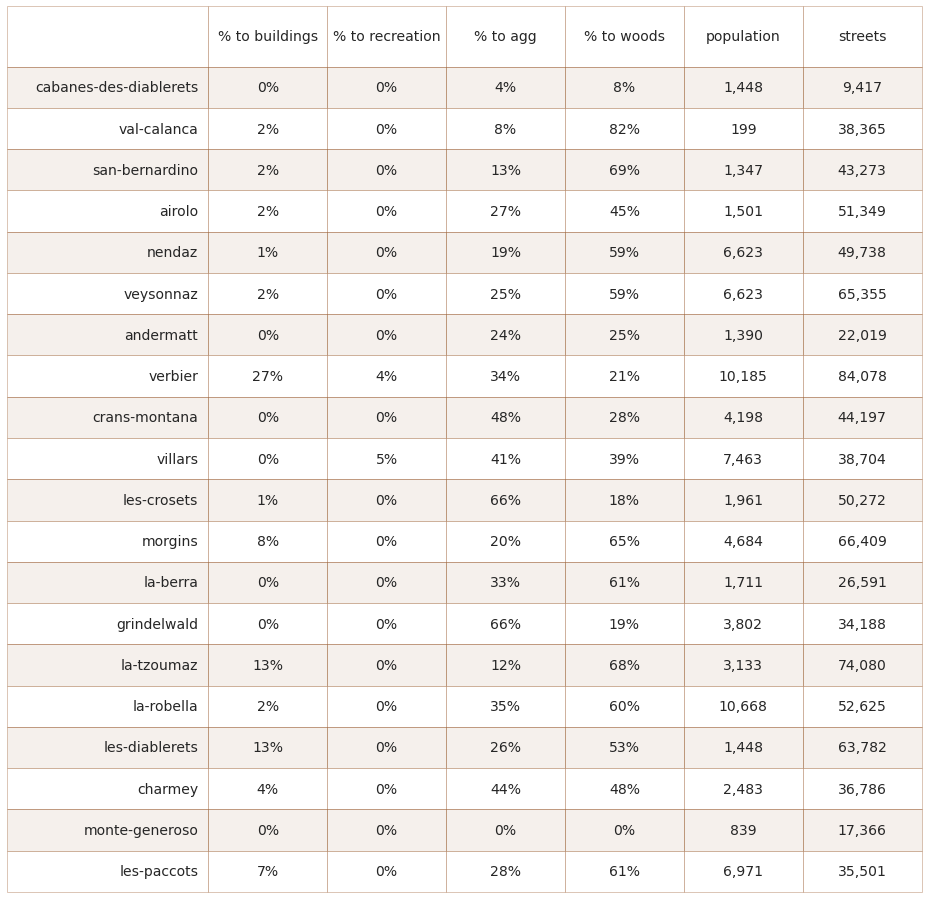
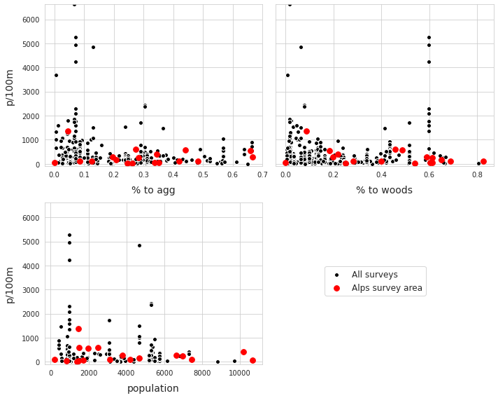
2.7.3. Les Alps with respect to land use¶

The results from AV are compared to the other survey results that have either % to woods or % to agg within the same range as AV. The ranges for AV are:

% to agg: 0 to 66%
% to woods: 0 to 83%
population: 199 to 10,668

# define land use ranges based on the sample data
this_range = (fd[l_f[0]].min(), fd[l_f[0]].max())
this_range_w = (fd[l_f[1]].min(), fd[l_f[1]].max())
this_range_p = (fd[l_f[2]].min(), fd[l_f[2]].max())

# apply them to all the data
# one test for agg -- a dominant land use feature of the sample data
some_data = a_data[(a_data[l_f[0]] >= this_range[0])&(a_data[l_f[0]] <= this_range[1])].copy()

# one test for woods -- the dominant land use feature of the sample data
some_data_w = a_data[(a_data[l_f[1]] >= this_range_w[0])&(a_data[l_f[1]] <= this_range_w[1])].copy()

# one test for population -- 
some_data_p = a_data[(a_data[l_f[2]] >= this_range_p[0])&(a_data[l_f[2]] <= this_range_p[1])].copy()

# remove Alps valaisannes
some_data = some_data[~some_data.location.isin(fd.location.unique())].copy()
some_data_w = some_data_w[~some_data_w.location.isin(fd.location.unique())].copy()
some_data_p = some_data_p[~some_data_p.location.isin(fd.location.unique())].copy()

# the number of samples and locations that have similar land use profiles as AV:
# agg to loc_date for each criteria
# data for charting and comparing
data=some_data.groupby(["loc_date","location",l_f[0]], as_index=False)[unit_label].sum()
data_w =some_data_w.groupby(["loc_date","location", l_f[1]], as_index=False)[unit_label].sum()
data_p = some_data_p.groupby(["loc_date","location",l_f[1], "population"], as_index=False)[unit_label].sum()
regional = fd.groupby(["loc_date","location", *l_f], as_index=False)[unit_label].sum()

# locations that share the characteristics
commonsamps = set(data.loc_date.unique()) & set(data_w.loc_date.unique())& set(data_p.loc_date.unique())
commonlocs = set(data.location.unique()) & set(data_w.location.unique())&set(data_p.location.unique())

# print these out to get the comparison

# print("agg")
# print(this_range)
# print(len(data.location.unique()))
# print(data.loc_date.nunique())
# print("woods")
# print(this_range_w)
# print(len(data_w.location.unique()))
# print(data_w.loc_date.nunique())
# print("p")
# print(this_range_p)
# print(len(data_p.location.unique()))
# print(data_p.loc_date.nunique())
# print(len(commonsamps))
# print(commonlocs)

# make a categorical df for mapping
mat_agg = dfBeaches.loc[data.location.unique()]
mat_agg["match"] = "agg"
mat_w = dfBeaches.loc[data_w.location.unique()]
mat_w["match"] = "woods"
mat_p = dfBeaches.loc[data_p.location.unique()]
mat_p["match"]="pop"

# merge all that and export to .csv
landusemap = pd.concat([mat_agg, mat_w, mat_p], axis=0)
# landusemap.to_csv("output/Alps-valaisannes/lu_comparison.csv", index=False)

Top left: survey total with respect to % to agg, range=(0%, 66%). Top right: survey total with respect to % to woods, range=(0%, 65%). Bottom left: survey total with respect to population, range=(199, 10,668)

fig, axs = plt.subplots(2,2, figsize=(10,8), sharey=True)

axone=axs[0,0]
axtwo=axs[0,1]
axthree=axs[1,0]
axfour=axs[1,1]

# plot the samples from all the data that meet the x criteria
sns.scatterplot(data=data, x="% to agg", y=unit_label, color="black", alpha=1, linewidth=1, label="All surveys", ax=axone, zorder=1)

# point estimates of the percentile ranking based off the edcf of all surveys
# place to store the rankings
rankings = {}

# plot the values for AV
for x in regional.location.unique():
    this_y = regional[regional.location == x][unit_label]
    this_x = regional[regional.location == x]["% to agg"]
    axone.scatter(this_x, this_y, color="red", s=60, zorder=2)

# handle extreme values
axone.set_ylim(0, max(data[unit_label].to_numpy()))

# set labels
axone.set_ylabel(unit_label, **ck.xlab_k14)
axone.set_xlabel("% to agg", **ck.xlab_k14)

# gather up legend handles
axone.get_legend().remove()

# start axtwo
# plot the samples from all the data that meet the x criteria
sns.scatterplot(data=data_w, x="% to woods", y=unit_label, color="black", alpha=1, linewidth=1, label="All surveys", ax=axtwo, zorder=1)

# plot the values from AV
for x in regional.location.unique():
    this_y = regional[regional.location == x][unit_label]
    this_x = regional[regional.location == x]["% to woods"]
    rankings.update({x:(this_x, this_y)})
    axtwo.scatter(this_x, this_y, color="red", s=60, zorder=2)

# handle extreme values
axtwo.set_ylim(0, max(data[unit_label].to_numpy()))

# set labels
axtwo.set_ylabel(unit_label, **ck.xlab_k14)
axtwo.set_xlabel("% to woods", **ck.xlab_k14)
axtwo.get_legend().remove()

# start axthree
# plot the samples from all the data that meet the x criteria
sns.scatterplot(data=data_p, x="population", y=unit_label, color="black", alpha=1, linewidth=1, label="All surveys", ax=axthree, zorder=1)

# plot the values from AV
for x in regional.location.unique():
    this_y = regional[regional.location == x][unit_label]
    this_x = regional[regional.location == x]["population"]
    rankings.update({x:(this_x, this_y)})
    axthree.scatter(this_x, this_y, color="red", s=60, label="Alps survey area", zorder=2)

# handle extreme values
axthree.set_ylim(-100, max(data[unit_label].to_numpy()))

# start axfour,# clear axfour
sut.hide_spines_ticks_grids(axfour)

# set labels
axthree.set_ylabel(unit_label, **ck.xlab_k14)
axthree.set_xlabel("population", **ck.xlab_k14)
handles, labels = axthree.get_legend_handles_labels()
axthree.get_legend().remove()

fig.legend(handles[:2], labels[:2], bbox_to_anchor=(.75,.25), loc="lower center",  fontsize=12)
plt.tight_layout()
plt.show()

2.7.4. Organisation and execution¶

Summit foundation: Téo Gürsoy

Hammerdirt: Bettina Siegenthaler

2.7.5. Survey locations¶

# display the survey locations
pd.set_option("display.max_rows", None)
disp_columns = ["latitude", "longitude", "city", "population", "streets", "% to buildings"]
disp_beaches = dfBeaches.loc[t["locations"]][disp_columns]
disp_beaches

	latitude	longitude	city	population	streets	% to buildings
slug
cabanes-des-diablerets	46.338604	7.215525	Ormont-Dessus	1448.0	9417.0	0.000000
val-calanca	46.330718	9.120103	Calanca	199.0	38365.0	0.021708
san-bernardino	46.445947	9.191344	Mesocco	1347.0	43273.0	0.022523
airolo	46.514257	8.607884	Airolo	1501.0	51349.0	0.027221
nendaz	46.162099	7.283486	Nendaz	6623.0	49738.0	0.019886
veysonnaz	46.180334	7.366005	Nendaz	6623.0	65355.0	0.024148
andermatt	46.618327	8.598803	Andermatt	1390.0	22019.0	0.000000
verbier	46.103981	7.224760	Val de Bagnes	10185.0	84078.0	0.271693
crans-montana	46.334214	7.479386	Lens	4198.0	44197.0	0.008439
villars	46.321937	7.073841	Ollon	7463.0	38704.0	0.008633
les-crosets	46.183591	6.832916	Val-d'Illiez	1961.0	50272.0	0.019886
morgins	46.236681	6.858132	Troistorrents	4684.0	66409.0	0.082504
la-berra	46.677399	7.178738	La Roche	1711.0	26591.0	0.001418
grindelwald	46.658523	8.065323	Grindelwald	3802.0	34188.0	0.005722
la-tzoumaz	46.144287	7.232897	Riddes	3133.0	74080.0	0.131915
la-robella	46.875905	6.548577	Val-de-Travers	10668.0	52625.0	0.029703
les-diablerets	46.346141	7.151228	Ormont-Dessus	1448.0	63782.0	0.136947
charmey	46.622641	7.189341	Val-de-Charmey	2483.0	36786.0	0.041311
monte-generoso	45.929625	9.019921	Rovio	839.0	17366.0	0.000000
les-paccots	46.512592	6.949421	Châtel-Saint-Denis	6971.0	35501.0	0.074074

2.7.6. Inventory of all items¶

pd.set_option("display.max_rows", None)
# code totals for the river bassin
fd_code_t= fd.groupby(["code", "groupname"], as_index=False).agg({"quantity":"sum", "fail":"sum", unit_label:"median"})
fd_code_t.rename(columns={"groupname":"utility"}, inplace=True)
fd_code_t["% of total"] = fd_code_t.quantity/fd_code_t.quantity.sum()
fd_code_t.set_index("code", inplace=True)
fd_code_t.sort_values(by="quantity", ascending=False, inplace=True)
fd_code_t["material"] = fd_code_t.index.map(lambda x: code_material_map[x])
fd_code_t["item"] = fd_code_t.index.map(lambda x: code_description_map.loc[x])
fd_code_t["% of total"] = (fd_code_t["% of total"]*100).round(1)
fd_code_t["fail rate"] = ((fd_code_t["fail"]/len(fd.loc_date.unique()))*100).round(1)
complete_inventory = fd_code_t[fd_code_t.quantity>0][["item", "quantity", "utility",  "% of total","fail rate"]]
complete_inventory

	item	quantity	utility	% of total	fail rate
code
G704	Brosse de télésiège	5181	infrastructure	66.6	10.0
G27	Cigarette filters	317	tobacco	4.1	95.0
Gfrags	Fragmented plastics	294	plastic pieces	3.8	50.0
G30	Food wrappers; candy, snacks	253	food and drink	3.3	95.0
G705	Screws and bolts	206	infrastructure	2.6	65.0
G936	Sheeting ag. greenhouse film	132	agriculture	1.7	15.0
Gfoam	Expanded polystyrene	121	infrastructure	1.6	0.0
G93	Cable ties; steggel, zip, zap straps	104	infrastructure	1.3	60.0
G200	Glass drink bottles, pieces	84	food and drink	1.1	45.0
G177	Foil wrappers, aluminum foil	68	food and drink	0.9	60.0
G124	Other plastic or foam products	60	unclassified	0.8	5.0
G941	Packaging films nonfood or unknown	57	packaging non food	0.7	30.0
G87	Tape, masking/duct/packing	53	infrastructure	0.7	60.0
G204	Bricks, pipes not plastic	49	infrastructure	0.6	40.0
G117	Expanded foams < 5mm	37	micro plastics (< 5mm)	0.5	5.0
G33	Lids for togo drinks plastic	36	food and drink	0.5	40.0
G12	Cosmetics, non-beach use personal care containers	34	personal items	0.4	5.0
G89	Plastic construction waste	34	infrastructure	0.4	15.0
G142	Rope , string or nets	33	recreation	0.4	40.0
G122	Plastic fragments ( >1mm)	32	micro plastics (< 5mm)	0.4	30.0
G919	Nails, screws, bolts etc.	31	infrastructure	0.4	20.0
G922	Labels, bar codes	27	packaging non food	0.3	40.0
G923	Tissue, toilet paper, napkins, paper towels	26	personal items	0.3	40.0
G703	piquet de ballisage	21	infrastructure	0.3	10.0
G24	Plastic lid rings	20	food and drink	0.3	35.0
G178	Metal bottle caps and lids	18	food and drink	0.2	40.0
G146	Paper, cardboard	18	packaging non food	0.2	25.0
G926	Chewing gum, often contains plastics	17	food and drink	0.2	25.0
G934	Sandbag, plastic for flood, erosion control etc..	17	agriculture	0.2	15.0
G10	Food containers single use foamed or plastic	17	food and drink	0.2	15.0
G34	Cutlery, plates and trays	16	food and drink	0.2	20.0
G25	Tobacco; plastic packaging, containers	16	tobacco	0.2	25.0
G905	Hair clip, hair ties, personal accessories pl...	16	personal items	0.2	40.0
G710	Ski / Snowboards (ski, fixations et autres piè...	15	recreation	0.2	30.0
G707	étiquette d’équipement de ski	13	recreation	0.2	25.0
G208	Glass or ceramic fragments > 2.5 cm	13	unclassified	0.2	25.0
G901	Mask medical, synthetic	13	personal items	0.2	20.0
G198	Other metal pieces < 50cm	12	infrastructure	0.2	40.0
G170	Wood (processed)	11	agriculture	0.1	10.0
G145	Other textiles	11	personal items	0.1	20.0
G152	Cigarette boxes, tobacco related paper/cardboard	11	tobacco	0.1	25.0
G7	Drink bottles < = 0.5L	11	food and drink	0.1	40.0
G709	Batons de ski parties (rondelles, attaches)	11	recreation	0.1	30.0
G66	Straps/bands; hard, plastic package fastener	10	infrastructure	0.1	10.0
G48	Rope, synthetic	10	recreation	0.1	20.0
G100	Medical; containers/tubes/ packaging	9	waste water	0.1	40.0
G31	Lollypop sticks	9	food and drink	0.1	25.0
G702	piquet de ballisage	9	infrastructure	0.1	20.0
G74	Insulation foams	8	infrastructure	0.1	0.0
G129	Inner tubes and rubber sheets	8	unclassified	0.1	5.0
G921	Ceramic tile and pieces	7	infrastructure	0.1	10.0
G105	Plastic fragments subangular <5mm	6	micro plastics (< 5mm)	0.1	5.0
G23	Lids unidentified	6	packaging non food	0.1	10.0
G20	Caps and lids	6	packaging non food	0.1	20.0
G156	Paper fragments	6	packaging non food	0.1	25.0
G123	Polyurethane granules < 5mm	6	micro plastics (< 5mm)	0.1	5.0
G918	Safety pins, paper clips, small metal utility ...	6	personal items	0.1	15.0
G706	Abonnement de ski	5	recreation	0.1	25.0
G149	Paper packaging	5	packaging non food	0.1	10.0
G191	Wire and mesh	5	agriculture	0.1	20.0
G943	Fencing agriculture, plastic	4	agriculture	0.1	10.0
G915	Reflectors, plastic mobility items	4	personal items	0.1	5.0
G175	Cans, beverage	4	food and drink	0.1	15.0
G73	Foamed items & pieces (non packaging/insulatio...	4	recreation	0.1	5.0
G211	Swabs, bandaging, medical	4	personal items	0.1	15.0
G35	Straws and stirrers	3	food and drink	0.0	15.0
G158	Other paper items	3	packaging non food	0.0	15.0
G95	Cotton bud/swab sticks	3	waste water	0.0	5.0
G171	Other wood < 50cm	3	agriculture	0.0	15.0
G194	Cables, metal wire(s) often inside rubber or p...	3	infrastructure	0.0	10.0
G712	Gants de ski	3	recreation	0.0	10.0
G711	Chaufferette	3	recreation	0.0	10.0
G139	Backpacks	3	personal items	0.0	5.0
G3	Plastic bags, carier bags	3	packaging non food	0.0	10.0
G159	Corks	3	food and drink	0.0	10.0
G210	Other glass/ceramic	2	unclassified	0.0	5.0
G90	Plastic flower pots	2	agriculture	0.0	10.0
G28	Pens, lids, mechanical pencils etc.	2	personal items	0.0	10.0
G928	Ribbons and bows	2	personal items	0.0	5.0
G931	Tape-caution for barrier, police, construction...	2	infrastructure	0.0	10.0
G713	Carpet from ski lift	2	infrastructure	0.0	5.0
G26	Cigarette lighters	2	tobacco	0.0	10.0
G155	Fireworks paper tubes and fragments	2	recreation	0.0	5.0
G181	Tableware metal; cups, cutlery etc.	2	food and drink	0.0	5.0
G167	Matches or fireworks	2	recreation	0.0	5.0
G168	Wood boards	2	agriculture	0.0	5.0
G935	Walking stick pads and pieces, often elastomer...	1	personal items	0.0	5.0
G71	Shoes sandals	1	personal items	0.0	5.0
G67	Industrial sheeting	1	agriculture	0.0	5.0
G148	Cardboard (boxes and fragments)	1	packaging non food	0.0	5.0
G65	Buckets	1	agriculture	0.0	5.0
G131	Rubber bands	1	personal items	0.0	5.0
G8	Drink bottles > 0.5L	1	food and drink	0.0	5.0
G128	Tires and belts	1	unclassified	0.0	5.0
G916	Pencils and pieces	1	personal items	0.0	5.0
G917	Terracotta balls	1	unclassified	0.0	5.0
G929	Electronics and pieces; sensors, headsets etc.	1	personal items	0.0	5.0
G21	Drink lids	1	food and drink	0.0	5.0
G708	Batons de ski	1	recreation	0.0	5.0
G195	Batteries - household	1	personal items	0.0	5.0
G101	Dog feces bag	1	personal items	0.0	5.0
G199	Other metal pieces > 50cm	1	infrastructure	0.0	5.0
G96	Sanitary-pads/tampons, applicators	1	waste water	0.0	5.0

The Alps and the Jura

Contents